Riemann zeta function on Re(s)>1
The clip begins by defining the function under study as the Dirichlet series for complex with . This is the starting object for the later discussion of analyticity.
黎曼的演算纸 · Bilibili · 18:56
This 160-second excerpt is a lecture-style introduction to analytic properties of the Riemann zeta function in the half-plane . It first states the series definition , then announces a proof plan: show that the partial sums converge uniformly on regions with fixed , and use the complex-analysis uniform limit theorem to conclude that is analytic. The clip also gives an informal description of analytic functions as continuous and infinitely differentiable, defines uniform convergence in words, introduces the partial-sum sequence , lists the first four examples, and ends by setting up a contrast between pointwise and uniform convergence. This 160-second lecture segment compares pointwise and uniform convergence of a sequence of functions ,, to a limit f. The left column defines pointwise convergence by first fixing a point x, then choosing , and asking for an index N such that implies ||<ε. The right column defines uniform convergence by first choosing and then requiring one N that makes the same inequality hold for all x in a region simultaneously. The lecturer highlights that the essential difference is the order of quantifiers and whether N may depend on x. The segment closes by applying this contrast to on : pointwise convergence was already shown previously, but uniform convergence on that whole region is stated to fail. This lecture segment analyzes the convergence of the partial sums of the Riemann zeta function, . It first confirms that the sequence of partial sums converges pointwise to for all . The core of the segment is a rigorous proof showing that this convergence is not uniform on the interval (1, ). By selecting a specific and choosing , the lecturer uses bounds derived from the integral test to demonstrate that the difference || can exceed regardless of how large n is chosen. The segment concludes by noting that uniform convergence can be restored by restricting the domain to for any fixed , thereby avoiding the singularity at . This lecture segment explores the uniform convergence of the partial sums of the Riemann zeta function. It first demonstrates why convergence is not uniform for real due to the singularity at , using a graphical counterexample. The instructor then formally defines uniform convergence for complex functions and introduces the concept of tail sums (or remainder sums) to analyze the difference between the zeta function and its partial sums. Finally, the segment begins the algebraic manipulation of the tail sum by expressing the complex variable s in terms of its real and imaginary parts, setting up the proof for uniform convergence on a restricted region Re(s) >= . This 160-second lecture excerpt analyzes the tail of the zeta Dirichlet series in the complex plane. It first rewrites +it and converts the summand into a real decay factor times a unit-modulus phase e^{-it()}. The speaker then applies the triangle inequality to obtain |(+it)| for . Next, for real , the terms are compared directly to get . Finally, the two estimates are chained by transitivity, and a shaded half-plane diagram summarizes the conclusion that in Re(s) the greatest value of || is achieved at the boundary point . This lecture segment focuses on proving the uniform convergence of the Riemann zeta function's partial sums in the complex plane. It begins by reviewing pointwise convergence and then constructs a rigorous proof that the convergence is uniform on the region where the real part of s is greater than or equal to 1 plus a positive constant a. The proof relies on bounding the remainder term at any complex point by its value at the real boundary. The segment concludes by introducing the Weierstrass M-test as a powerful theorem that could simplify such proofs, explaining its conditions and utility in complex analysis. This lecture segment introduces key concepts from complex analysis to prove that the Riemann zeta function is analytic for Re(s) > 1. It begins by mentioning the Weierstrass M-test as a tool for establishing uniform convergence. The speaker then explains why uniform convergence is crucial, as it permits operations like interchanging limits with integrals and derivatives. Next, the concept of analytic functions is defined as a strong condition implying infinite differentiability. Several examples of analytic functions are listed, including polynomials, trigonometric functions, exponentials, and the individual terms of the zeta series. The core of the segment is the application of the Uniform Limit Theorem: since the partial sums of the zeta series are finite sums of analytic functions (and thus analytic themselves), and they converge uniformly to the zeta function on regions Re(s) >= , the limit function (the zeta function) must also be analytic. Because 'a' can be arbitrarily small, this proves analyticity on the entire open half-plane Re(s) > 1, which is visually summarized with a shaded region on the complex plane. This short closing segment previews the next lessons on the Riemann zeta function. On screen, text states that is analytic on , while a complex-plane diagram shades that right half-plane in green and shows a moving red point. The narration says the series will first study zeta’s behavior in this region before extending it to the rest of the complex plane.
Use the learning inspector for key ideas and moments, or open the reading tabs for the complete notes.
Generated from the video's visuals and explanation; not verbatim speech.
The clip opens with a title card naming the topic as analytic properties of the zeta function in the half-plane .
The first content slide defines the object of study directly: for complex with , . The speaker reads this formula and states that the episode will examine analytic properties of in this region.
The lecture then announces the first major step of the argument. Instead of trying to work all the way up to the boundary line , it fixes a positive constant and targets uniform convergence on the closed half-plane . The spoken explanation ties this choice to avoiding the blow-up near real part one.
Next, the slide introduces the complex-analysis tool that will convert convergence into regularity: if a sequence of analytic functions converges uniformly to , then is analytic in a domain. Alongside that theorem, the lecture gives an informal picture of analyticity by listing consequences such as continuity and infinite differentiability.
A new slide titled Convergence defines uniform convergence in words as convergence of a sequence of functions to a limit function at the same rate across the entire region. This is still an informal definition rather than a formal epsilon-based statement.
The abstract notion is then specialized to the zeta series. The sequence under consideration is the partial sums . The speaker explicitly explains the notational shift: now labels the sequence element, while is the dummy summation index inside the finite sum.
To make the definition concrete, the slide writes out the first four members of the sequence: , , , and . These are exactly the truncations of the zeta series after one, two, three, and four terms.
The final seconds switch to a comparison slide with two headings, pointwise convergence of to and uniform convergence of to . The speaker says they will describe what uniform convergence is, but the actual side-by-side explanation has not yet begun within this excerpt.
The segment opens on a slide titled “Convergence,” with two parallel headings: “Pointwise convergence of , , ..., to f” on the left and “Uniform convergence of , , ..., to f” on the right. The lecturer says the easiest way to understand the new topic is to compare it with pointwise convergence, which students may already have encountered informally.
The left column is then built in order. First comes “First pick a point x.” Next comes “Then pick .” Finally the slide asks: “Is there an index N such that whenever , || < ε?” The spoken explanation matches this sequence: fix a particular input point, choose a tolerance, and then look for a threshold index that makes the function values close to the limit at that fixed point.
Attention shifts to the right column for uniform convergence. The lecturer explicitly notes that the order changes. The slide now begins with “First pick ,” and then asks whether there is an index N such that whenever , the inequality || < ε holds “for all x in a region?” The same algebraic inequality appears, but the quantifier structure is different because x has not been fixed in advance.
The phrase “for all x in a region?” is visually emphasized, underscoring the universal quantifier over the whole domain. The lecturer calls this the key difference: in the uniform case, one single N must work simultaneously for every x in the region, rather than separately at each point.
Two summary bullets appear at the bottom to crystallize the contrast. On the left: “N can be chosen dependent on x.” On the right: “N must be chosen for all x simultaneously.” This is the operational distinction between the two definitions: pointwise convergence allows the threshold to vary with the point, while uniform convergence forbids that dependence.
The final bullets apply the definitions to the Riemann zeta function on the real domain . The left note says, “We already showed this is true for when ,” referring back to an earlier integral-test argument. The right note says, “As we'll see, this is false for when .” Thus the clip ends by setting up a concrete example where pointwise convergence holds but uniform convergence on the whole region does not.
We begin by defining the partial sums of the Riemann zeta function: , , and in general, . As established previously, this sequence of functions converges pointwise to for all .
Next, we investigate whether this convergence is uniform on the interval (1, ). To disprove uniform convergence, we must find an such that for any N, there exists an and an where || . We choose .
First, observe that for any , each term in the partial sum is less than or equal to 1. Since there are n terms, we have the upper bound .
The key insight is to exploit the behavior of near its singularity at . We choose a specific x that depends on n: . As n grows, this x gets arbitrarily close to 1 from the right.
Using a result from the integral test, we know that . This provides a lower bound for the limit function at our chosen x.
Now we evaluate the difference: ||. Substituting our bounds, we get || > () - . Since , the condition for uniform convergence fails.
Therefore, the sequence does not converge uniformly to on the entire domain . The root cause is that we were able to pick an x arbitrarily close to 1, where the gap between the partial sum and the limit function becomes large.
However, if we restrict our attention to a smaller domain, specifically for some fixed , we stay away from the singularity. On this restricted interval, the sequence does converge uniformly to .
The segment begins by analyzing the uniform convergence of the partial sums of the Riemann zeta function, , for real values . A graph illustrates the function and a partial sum . As x approaches 1, exhibits a vertical asymptote, growing arbitrarily large. The instructor explains that this singularity prevents uniform convergence on the entire domain . A specific counterexample is provided: by choosing and selecting , the value of can be made greater than , while the partial sum is bounded by n. This results in || > , violating the condition for uniform convergence.
To address this, the lecture transitions to complex analysis and formally defines uniform convergence for a sequence of complex functions converging to on a region A. The definition states that for any given , there must exist an integer N such that for all , the inequality || < holds simultaneously for all points z in A. The instructor then defines the partial sums and introduces the concept of tail sums, or remainder sums, denoted as . The tail sum is defined as the difference between the full zeta function and the partial sum: This formula needs review. Please report it using the page feedback control.infty . The goal is now to prove that converges uniformly to on a restricted region for some fixed , which effectively keeps the domain away from the singularity at . This is achieved by showing that for any , there exists an N such that || < for all and all s in the region.
The final part of the segment focuses on algebraically manipulating the tail sum to facilitate the proof. The complex variable s is expressed in its standard form, + it, where is the real part and t is the imaginary part. Substituting this into the tail sum yields This formula needs review. Please report it using the page feedback control.infty . Using the properties of exponents, the denominator is split into ^{it}, resulting in This formula needs review. Please report it using the page feedback control.infty ^{-it}. The term k is then rewritten as , transforming the expression to This formula needs review. Please report it using the page feedback control.infty ^{-it}. Finally, applying the power of a power rule for exponents, the expression simplifies to This formula needs review. Please report it using the page feedback control.infty ^{-it()}. This manipulation separates the magnitude and phase components of the terms in the tail sum, setting the stage for bounding the sum to prove uniform convergence.
The clip opens on a slide titled “Zeta in the Complex Plane.” The first mathematical move is purely notational: the complex argument is written as . With that substitution, the tail of the Dirichlet series is displayed as . The speaker stresses that this is not the full sum from , but a tail beginning at .
The next lines rewrite the summand step by step. First becomes , then it splits as . Moving the oscillatory factor to the numerator gives . Because the speaker says “log base e” is being used, is rewritten as , so . Thus the tail takes the form , separating size from phase.
A new slide assumes and estimates the modulus of this complex tail. The key inequality is the triangle inequality: the absolute value of a sum is at most the sum of the absolute values. Applying it termwise gives . Since is positive real and , the right-hand side collapses to . The speaker’s verbal image is that the terms are vectors spiraling around rather than all pointing in the same direction, so cancellation can only make the true modulus smaller.
The argument then shifts from complex inputs to real inputs. Under the hypothesis “For real ,” the slide writes out the first few terms of and and compares them term by term. Because and the bases are positive, one has . Taking reciprocals reverses the inequality, yielding . Summing these inequalities over the same index set gives .
The final slide combines the two previous estimates and adds a geometric picture. On the left, the complex plane is drawn with Real and Imaginary axes, the vertical boundary line at , and a shaded half-plane consisting of all points with . A sample point is marked inside this region, with its projection on the real axis. On the right, the inequalities are chained: and . By transitivity, every point in the half-plane satisfies . Since equality is attained at the boundary point , the slide concludes that the greatest value of in the region occurs there.
The lecture resumes with a slide titled 'Zeta in the Complex Plane'. The speaker notes the similarity to a previous episode, clarifying that the current focus is on the remainder term rather than the full zeta function .
The goal is to complete the proof regarding the convergence of the series. The speaker recalls that the partial sums are already known to converge pointwise to for , a result established via the integral test in a prior session.
To bridge pointwise and uniform convergence, the speaker fixes a specific point on the real axis: , where . By the definition of pointwise convergence, for any arbitrary , there exists an integer such that for all , the difference —which equals the remainder —is strictly less than .
Crucially, the speaker proposes using this same and the same threshold for the entire region defined by . The logic is that if the error is small at the boundary 'worst-case' point, it should be small everywhere inside the region.
The derivation proceeds by taking an arbitrary complex number in the region, meaning . The magnitude of the remainder is bounded. First, it is noted that , implying the error is maximized when the imaginary part is zero. Second, since and the remainder function decreases as the real argument increases, .
Combining these inequalities yields . Since represents the distance between the partial sum and the limit function , this inequality holds for all in the region using the single derived earlier.
This satisfies the formal definition of uniform convergence. The speaker concludes that the sequence of partial sums converges uniformly to on the region .
The slide transitions to a new topic: 'Complex Analysis'. The speaker introduces the Weierstrass M-test as a standard theorem that offers a faster route to proving uniform convergence, though he chose the manual derivation to build intuition.
The Weierstrass M-test is stated: If you have an infinite series of functions defined on a region , and if each function's magnitude is bounded by a constant (i.e., for all ), and if the series of these constants converges, then the original series of functions converges uniformly on .
The speaker reflects that this test could have been applied directly to the zeta function problem to skip the detailed bounding steps, but emphasizes the value of understanding the underlying mechanics of convergence definitions.
The lecturer begins by referencing the Weierstrass M-test, a theorem from complex analysis used to establish uniform convergence of infinite series of functions. The slide displays the formal statement: if the absolute value of each function is bounded by a constant , and the series of these constants converges, then the original series converges uniformly in the specified region.
Addressing the question of why uniform convergence is so important, the speaker explains that it grants permission to perform critical calculus operations. Specifically, it allows mathematicians to safely interchange the order of limits with summations, integrations, and differentiation, which is essential for manipulating complex series.
The focus shifts to the concept of analytic functions. The speaker defines 'analytic' as a condition significantly stronger than mere continuity or differentiability. In the context of complex analysis, an analytic function is exceptionally well-behaved, implying it is infinitely differentiable and can be locally represented by a convergent power series.
To illustrate, several common analytic functions are listed on the slide. These include polynomials like , the trigonometric function , and the exponential function . The lecturer also points out that the individual terms of the Riemann zeta series, , are analytic functions of the complex variable .
The pivotal tool for the upcoming proof is introduced: the Uniform Limit Theorem. The slide states that if a sequence of analytic functions converges uniformly to a limit function within a domain, then that limit function must also be analytic in that domain.
Applying this theorem to the Riemann zeta function, the lecturer constructs a logical proof. First, the partial sums are identified as finite sums of analytic functions, making them analytic themselves. Second, because the series converges uniformly on regions where (for any ), the Uniform Limit Theorem dictates that the limit function, , is analytic on these regions.
Since the parameter can be chosen to be arbitrarily small, the union of all such regions covers the entire open half-plane where . Consequently, the proof concludes that the Riemann zeta function is analytic everywhere to the right of the vertical line in the complex plane.
The segment ends with a visual summary. A diagram of the complex plane is shown, with a green shaded region extending to the right of the dashed vertical line at . This visually reinforces the main takeaway: the zeta function is highly regular and analytic throughout this specific domain.
The right side of the screen directly presents the key conclusion: The function zeta of s is analytic, that is, very well behaved, on the region where the real part of s is greater than one. Here, s is a complex variable, and the real part of s denotes its real component, so the condition real part of s is greater than one describes the open right half-plane in the complex plane lying to the right of the vertical line real part of s equals one.
The left-side diagram geometrizes this condition: the horizontal axis is labeled Real, the vertical axis is labeled Imaginary, the origin is zero, the point one is marked on the horizontal axis, and a vertical dashed line passes through one. The green shaded region is exactly where the real part of s is greater than one. A small red dot moves within this region to represent the complex point s currently under consideration.
The narrator then outlines the course plan: in the next few videos, we will first discuss zeta's behavior in this region—that is, study zeta of s within the known analytic right half-plane. The purpose of this step is to first understand the function in a region where it has favorable properties, before tackling the more challenging extension problem.
Next, the narrator notes that several more videos will be devoted to this topic before zeta is truly extended to the rest of the complex plane. Correspondingly, in the animation, the red dot crosses the dashed line into the left non-green region, visually representing the shift from the region where the real part of s is greater than one to the rest of the complex plane.
Thus, although this segment is brief, it clearly establishes two layers: first, zeta of s is analytic where the real part of s is greater than one; second, the upcoming study will first focus on this region, then address extension to the full complex plane. The video does not prove analyticity here, but treats it as the starting point for the next series of discussions.
The clip begins by defining the function under study as the Dirichlet series for complex with . This is the starting object for the later discussion of analyticity.
The lecture plans to prove uniform convergence not on the whole half-plane , but on a shifted closed region with fixed . The spoken reason is to stay away from the singular behavior near real part one.
After uniform convergence is established, the video invokes a standard complex-analysis result: a uniform limit of analytic functions is analytic. This is the bridge from convergence of partial sums to analyticity of the zeta function.
The clip does not give a formal definition of analyticity here. Instead it describes analytic functions as especially well behaved and lists immediate consequences such as continuity and infinite differentiability.
Uniform convergence is introduced as convergence of a sequence of functions to a limit function at the same rate across the entire region. This verbal definition prepares the viewer for the later contrast with pointwise convergence.
The specific sequence being studied is the finite truncation of the zeta series: . The speaker explains that is used inside the sum because already labels the sequence element.
The slide makes the abstract definition concrete by writing the first four terms of the sequence. Each new adds exactly one more reciprocal power term from the zeta series.
The last visible slide creates a two-column comparison between pointwise convergence and uniform convergence for a generic sequence tending to . Within this excerpt, only the headings appear; the detailed comparison has not yet started.
Pointwise convergence is defined by fixing a point x first, then choosing , and asking whether there exists an index N such that for all one has ||<ε. Because x is already chosen, N may depend on that particular point.
Uniform convergence reverses the initial order of choices: first pick , then ask for a single index N such that whenever , the inequality ||<ε holds for all x in the region at the same time.
The clip stresses that the two definitions look similar because both use ||<ε, but they differ fundamentally in quantifier order. Pointwise convergence is ∀x ∀ε ∃N, while uniform convergence is ∀ε ∃N ∀x. That change is what makes uniform convergence stronger.
The practical distinction summarized on the slide is that in pointwise convergence, N can be chosen dependent on x, whereas in uniform convergence, N must be chosen for all x simultaneously. This is the key diagnostic difference between the two notions.
Applying the definitions to the Riemann zeta function on real inputs , the lecturer recalls that pointwise convergence was already shown previously using the integral test, but states that uniform convergence on the whole region will fail.
The sequence of partial sums converges pointwise to the Riemann zeta function for every . This means that for any fixed x in this domain, the numerical sequence approaches as n goes to infinity.
To show that does not converge uniformly to on (1, ), we fix . For any n, we choose . Using the bounds and (from the integral test), we find || > . Since this holds for arbitrarily large n, uniform convergence fails.
While uniform convergence fails on the full interval (1, ) due to the singularity at , it can be recovered by restricting the domain. If we choose any fixed and consider the interval [, ), the sequence converges uniformly to . This is because we are bounded away from the problematic point .
A sequence of complex functions converges uniformly to f on a region A if for every , there exists an N such that for all , || < for all z in A simultaneously.
The n-th partial sum of the Riemann zeta function series is defined as the sum of the first n terms.
The n-th tail sum represents the remaining infinite series after subtracting the first n terms from the full zeta function.
The partial sums do not converge uniformly to for because the singularity at causes to grow arbitrarily large, making it impossible to bound the difference || by a single epsilon across the entire domain.
To analyze the tail sum for complex s, substitute + it and apply exponent rules to separate the real and imaginary components.
The clip studies the tail of the zeta Dirichlet series, defined by starting the sum at rather than at . This distinction is repeated verbally and visually throughout the excerpt.
The standard decomposition +it is introduced so that the real part controls magnitude and the imaginary part controls oscillation in each summand.
Using the natural logarithm, k is rewritten as . This turns k^{-it} into e^{-it()}, giving a clean separation between the decaying factor and a pure phase.
Explore conditions, steps and evidence. Supplementary explanations are labeled separately from content shown in the video.
Slide text and displayed formula use for the Riemann zeta function.
The speaker says the Riemann zeta function is defined as the sum from n equals one to infinity of one over n to the s.
The Riemann zeta function in the half-plane under discussion.
Defined on complex numbers with in this clip.
The slide states that the function is defined for complex numbers with .
The speaker explicitly says the definition is for complex numbers with real part greater than one.
s
Complex argument of the zeta function.
for the definition; later restricted to for uniform convergence discussion.
The slide displays and .
The speaker refers to the real part of being greater than one and then greater than or equal to .
Real part of the complex number .
Real-valued quantity associated with .
The infinite series is written as .
The speaker says the sum runs from to infinity.
n
Summation index in the infinite series defining , and also the sequence index for partial sums in this clip.
Positive integers.
The partial-sum formula is written as .
The speaker says he is using instead of because is already used for the sequence of functions.
k
Dummy summation index inside the finite partial sum.
Positive integers with in .
The slide states uniform convergence in .
The speaker says to pick a number greater than zero first and fix that number.
a
A fixed positive constant used to stay away from the boundary at real part one.
.
The slide defines .
The speaker says the partial sums are going to be these , which only sum from to .
The th partial sum of the zeta series.
Defined for the same complex as the zeta series under discussion.
The comparison slide writes converging to .
The speaker says uniform convergence is when a sequence of functions converges to a limit function.
,,
Generic notation for a sequence of functions and its limit function.
Used abstractly in the convergence comparison slide.
Slide text shows “, , ..., to f” under both “Pointwise convergence” and “Uniform convergence”.
, ,
A sequence of functions being compared for convergence.
Functions on a region; in the later example, real x with .
Slide text says convergence “to f”.
The lecturer reads the difference ||.
f
The limiting function to which the sequence is converging.
A function defined on the same region as the .
Left bullet: “First pick a point x.”
“you first pick a point x”.
x
A chosen input point for pointwise convergence; in uniform convergence it ranges over all x in a region.
A point in the domain/region under discussion.
Bullets show “Then pick ” and “First pick ”.
“pick an epsilon greater than zero”.
A positive tolerance used in the epsilon-N definition of convergence.
Positive real numbers, .
Slide title and body state: The Riemann zeta function is defined for complex numbers with as .
The speaker reads the definition aloud and says today they will cover analytic properties of in this region.
In this clip, the zeta function is introduced by its Dirichlet-series definition on the open half-plane where the real part of exceeds one. The speaker frames the rest of the lesson around analytic properties of this function in that region.
is complex
Slide bullet says: We'll show that the partial sums converge uniformly in .
The speaker says the first thing they will show is that the partial sums converge uniformly in the region real part of greater than or equal to , and explains choosing to avoid the singularity near real part one.
The lecture sets up a proof strategy: first establish uniform convergence of the partial sums on a closed half-plane shifted away from the boundary line . The parameter is fixed so the region stays a positive distance from the problematic boundary.
is fixed
the statement concerns the partial sums of
Slide bullets say: Uniform convergence allows to invoke the uniform limit theorem in complex analysis: If is a sequence of analytic functions converging uniformly to , then is analytic (in a domain). Analytic continuous, infinitely differentiable, etc.
The speaker says once they have uniform convergence they will use a theorem from complex analysis to show zeta is analytic, and describes an analytic function as very well behaved: continuous, smooth, differentiable, in fact infinitely differentiable.
The video does not give a formal epsilon-delta or power-series definition of analyticity here; instead it characterizes analytic functions informally as especially well-behaved functions and lists consequences such as continuity and infinite differentiability. This is paired with the announced plan to prove analyticity via a uniform limit theorem.
used as informal lecture characterization in this clip
Convergence slide states: Uniform convergence is when a sequence of functions converges to the limit function at the same rate across the entire region.
The speaker reads essentially the same sentence aloud.
The clip introduces uniform convergence as convergence of a sequence of functions to a limit function at the same rate throughout the whole region, rather than point by point with possibly different local behavior.
sequence of functions
limit function
entire region
Slide states: In this case, our sequence is the partial sums of , i.e. .
The speaker says the sequence they will deal with is the sequence of partial sums of zeta, and explains using instead of because indexes the sequence of functions.
The function sequence used in the convergence discussion is defined explicitly as the finite truncations of the zeta series. The index change from to inside the sum is explained verbally to avoid collision with the outer sequence index.
is a positive integer
runs from to
Slide lists , , , .
The speaker says here are the first few partial sums and describes as just one and as one plus one over two to the s.
The lecture writes out the first four members of the sequence to make the abstract definition concrete. These examples show how each new partial sum adds exactly one more term of the zeta series.
directly displayed on the slide
Left column lists: “First pick a point x.”; “Then pick .”; “Is there an index N such that whenever , || < ε?”
Lecturer explains the same order: pick x, then epsilon, then find N depending on that point.
Pointwise convergence is presented as a three-step test at a fixed point: first choose a point x, then choose a tolerance , then ask whether there exists an index N such that for every the value is within ε of . The lecturer emphasizes that because x has already been fixed, the required N may depend on that chosen point.
A sequence of functions ,, and a limiting function f are given.
The definition is applied at a fixed point x.
ε is any positive real number.
N may depend on x.
Right column lists: “First pick .”; “Is there an index N such that whenever , || < ε for all x in a region?”
“So we're first going to pick an epsilon greater than zero. So notice we're not picking a point.”
Uniform convergence is introduced by changing the order of quantifiers relative to pointwise convergence. Instead of first fixing a point x, one first chooses and then asks for a single index N that makes ||<ε hold simultaneously for every x in the region.
A sequence of functions ,, and a limiting function f are given.
The condition must hold for all x in the specified region at the same time.
ε is chosen before x is considered.
One N must work uniformly across the region.
Bottom bullets state “N can be chosen dependent on x” and “N must be chosen for all x simultaneously”.
“in the pointwise convergence, you can pick an N dependent on x, whereas for uniform convergence, the N has to be chosen for all x simultaneously.”
The clip identifies the key practical distinction between the two notions: in pointwise convergence the threshold index N is allowed to vary with the chosen point x, while in uniform convergence a single N must serve all points in the region at once. This is the central comparison used to motivate why pointwise convergence does not automatically imply uniform convergence.
Comparing the same sequence and limit f on a region.
Pointwise: N may depend on x.
Uniform: one N works for all x in the region.
so converges pointwise to , .
And we already know that f sub n of x converges pointwise to zeta of x because we showed that this infinite series does converge.
The sequence of partial sums converges pointwise to the Riemann zeta function for all . This means that for any fixed , the limit of as n approaches infinity is .
|| > , so is not uniformly convergent for .
And therefore, f sub n is not uniformly convergent for x greater than one.
To prove that does not converge uniformly to on the interval (1, ), one must show there exists an such that for any N, there is an and an where || . The video constructs this by choosing and .
Domain is
The sequence is uniformly convergent to if we first choose an , then set our region to .
If the domain is restricted to for some fixed , the sequence of partial sums converges uniformly to . This avoids the singularity at that causes the failure of uniform convergence on the larger domain.
Slide text states: If is a sequence of analytic functions converging uniformly to , then is analytic (in a domain).
The speaker says they will use a theorem from complex analysis once they have uniform convergence to show that zeta is analytic.
The clip states the theorem but does not prove it here.
The precise hypotheses beyond analyticity of the and uniform convergence are not expanded in this excerpt.
If is a sequence of analytic functions converging uniformly to , then is analytic in a domain.
is a sequence of analytic functions
converges uniformly to
For a sequence of analytic functions and its uniform limit in the stated setting.
Slide text states: Analytic continuous, infinitely differentiable, etc.
The speaker says an analytic function is continuous, smooth, differentiable, and in fact infinitely differentiable.
The slide uses 'etc.' without enumerating further consequences in this clip.
Analytic functions are continuous and infinitely differentiable.
The function is analytic
Stated as a general implication in the lecture slide.
Slide bullet states: We'll show that the partial sums converge uniformly in .
The speaker says the first thing they will show is that the partial sums converge uniformly in that region.
This excerpt announces the goal but does not yet carry out the proof.
The partial sums of converge uniformly in the region .
is fixed
the functions are the partial sums of the zeta series
For the partial-sum sequence introduced in the clip, on the half-plane .
Bottom-left green bullet: “We already showed this is true for when .”
Bottom-right red bullet: “As we'll see, this is false for when .”
“we've shown that zeta of x ... just does pointwise converge if x is greater than one. And as we'll see, this is actually not uniformly convergent for zeta of x when x is greater than one.”
The proof itself is not contained in this clip; it is referenced as having been shown in a previous episode using the integral test.
For the sequence discussed in connection with , the clip states that pointwise convergence holds when , but uniform convergence on that same region fails.
The functions under discussion are those associated with .
The region considered is .
Pointwise convergence was previously established by an integral-test argument.
Pointwise: for each fixed and each there exists N (possibly depending on x). Uniform: the claim is that no single N works for all simultaneously.
“the order of doing these things is going to be a little bit different.”
Left column begins with “First pick a point x.” while right column begins with “First pick .”
The clip presents the difference between pointwise and uniform convergence as arising from the order in which x and ε are chosen: pointwise fixes x first, uniform fixes ε first and then requires the condition for all x.
A sequence of functions and a limit function f are given on a region.
Pointwise: ∀x ∀ε ∃N. Uniform: ∀ε ∃N ∀x.
(by the result from our integral test earlier).
And by the integral test that we did in the previous episode, we showed that zeta of one plus one over n plus one, this infinite series is at least or in fact it's strictly greater than n plus one.
For any positive integer n, .
n is a positive integer
Note that , since each term of the sum is at most 1.
Then the value of f sub n of x, and I'm only looking at real numbers here, is at most n... each term's the one is at most one, one over two to the x is at most one, and one over three to the x is also at most one.
For any and any positive integer n, .
n is a positive integer
,
so is not uniformly convergent for .
The sequence of partial sums is not uniformly convergent to for .
are the partial sums of
Consider the region Re(s) , for fixed . We just need to show that given , we can find an N such that for all , || < for all s in the region.
The sequence is uniformly convergent to if we first choose an , then set our region to .
Second slide explicitly writes |(+it)| under the heading For .
Speaker says the absolute value of (+it) is at most equal to at .
For , the modulus of the complex tail satisfies |(+it)|.
+it.
.
.
For the displayed and corresponding complex +it.
Third slide states For real and concludes .
Speaker says therefore is at most .
If and are real and , then .
.
.
.
For real satisfying .
Final slide states Hence, in the region Re(s), the greatest value of || is achieved at .
Speaker says if I take an arbitrary point in this region, then the absolute value at that point is at most the value of at .
The slide asserts where the greatest value is achieved, but the clip does not separately prove existence beyond the displayed finite-tail inequality chain.
In the region Re(s), the greatest value of || is achieved at .
+it.
Re(s)=.
The previously shown bounds |(+it)| and hold.
For all s in the half-plane Re(s).
The speaker lays out the order: first show uniform convergence of the partial sums in , then use a theorem from complex analysis to conclude zeta is analytic.
The slide bullets present the same sequence of steps and the uniform limit theorem statement.
Only the outline is given in this clip; the actual convergence proof is not performed before 160 seconds.
Start from the definition on .
Directly shown on the opening slide and read aloud.
Restrict attention to a smaller closed region with fixed .
The speaker explains this avoids approaching the singularity at real part one.
Show that the partial sums converge uniformly on that region.
This is explicitly announced as the first main step on the slide and in speech.
Apply the uniform limit theorem from complex analysis to conclude the limit function is analytic.
The slide states the theorem and the speaker says this is the next step after uniform convergence.
The clip presents a two-step strategy: prove uniform convergence of the zeta partial sums away from the boundary, then invoke the uniform limit theorem to obtain analyticity of .
Side-by-side slide builds left column first, then right column, then adds bottom comparison bullets.
Lecturer explicitly contrasts “First pick a point x” with “First pick ” and then says the key difference is that N must apply for all x simultaneously.
The left column starts by fixing a particular input point before any tolerance is chosen.
Directly shown on the slide and read aloud.
After x is fixed, a positive tolerance is selected.
Directly shown on the slide and read aloud.
For that fixed x, one asks whether some threshold index N forces the values to stay within ε of .
This is the displayed pointwise condition.
The right column reverses the initial order by choosing the tolerance before considering points.
Directly shown on the slide and emphasized verbally.
One N must make the inequality true simultaneously across the whole region.
This is the displayed uniform condition.
The concluding comparison bullets state the operational difference between the two definitions.
Explicit bottom bullets and spoken summary.
Pointwise and uniform convergence differ because the quantifier order changes: fixing x first allows N to depend on x, while fixing ε first requires a single N valid for every x in the region.
Green bullet says pointwise statement is already true for when .
Red bullet says the uniform statement will be false for when .
Lecturer references a previous episode and the integral test, then says he is now dealing with real functions .
The actual integral-test computation and the precise sequence defining are not shown in this clip.
The clip references prior material rather than reproducing it.
The lecturer recalls that convergence for real part greater than one was shown earlier by an integral-test argument.
Spoken reference to prior content; not re-derived here.
He states that in this clip he is only plugging in real values to make the discussion easier.
Audio explanation accompanying the slide text when .
The green bullet records the already-established pointwise fact.
Explicit slide statement plus spoken recap.
The red bullet announces the upcoming contrast with the uniform definition.
Explicit slide statement plus spoken preview.
Using previously established pointwise convergence of for , the clip sets up the next step: showing that the stronger uniform condition does not hold on that whole region.
Suppose we pick an , say 0.005. Note that ... Then we can pick a number small enough such that ... Then || > , so is not uniformly convergent for .
Choose a specific positive value for epsilon.
Definition of non-uniform convergence requires finding at least one epsilon.
Establish an upper bound for the partial sum .
Each term is less than or equal to 1 for , and there are n terms.
Choose a specific value for x that depends on n and approaches 1 as n increases.
This choice exploits the singularity of at .
Establish a lower bound for the zeta function at the chosen x.
By the integral test result cited in the video.
Combine the bounds to estimate the difference between the limit function and the partial sum.
Substituting the bounds into the absolute difference expression.
Show that the estimated difference is strictly greater than the chosen epsilon.
Numerical comparison.
Conclude that the condition for uniform convergence fails.
By definition, since there exists an epsilon for which no single N works for all .
The sequence of partial sums does not converge uniformly to on the interval (1, ).
This formula needs review. Please report it using the page feedback control.infty This formula needs review. Please report it using the page feedback control.infty This formula needs review. Please report it using the page feedback control.infty This formula needs review. Please report it using the page feedback control.infty ^{-it} = This formula needs review. Please report it using the page feedback control.infty ^{-it} = This formula needs review. Please report it using the page feedback control.infty ^{-it()}
Start with the definition of the tail sum.
Definition of
Substitute + it.
Standard notation for complex variable s
Use exponent rules to split the denominator.
Algebraic property of exponents:
Move the term with it to the numerator by changing the sign of the exponent.
Algebraic property of exponents:
Rewrite k as .
Identity: for
Apply exponent rules to combine the exponents.
Algebraic property of exponents: ()^^{bc}
The tail sum can be expressed as This formula needs review. Please report it using the page feedback control.infty ^{-it()}.
First slide shows the full chain from to ^{-it()}.
Speaker notes the use of log base e and .
Start from the definition of the tail series.
Displayed definition on the slide.
Substitute the standard notation +it into the exponent.
Slide text states +it.
Split the power using the law .
Algebraic exponent rule shown implicitly by the displayed equality.
Move the factor k^{it} from the denominator to a negative exponent in the numerator.
Reciprocal rule ^{-it}.
Rewrite k as using the natural logarithm.
Speaker explicitly says log base e is being used and .
Combine the exponents to obtain the standard oscillatory factor.
Power-of-exponential rule ()^^{ab}.
The tail can be written as (+it)=^{-it()}.
Second slide displays the chain |(+it)|=| ...| |...|=.
Speaker identifies this as the triangle inequality and describes the terms as vectors spiraling rather than aligning.
Insert the exponential form of the tail obtained previously.
Uses the prior derivation of the rewritten series.
Bound the modulus of the sum by the sum of the moduli.
Triangle inequality, explicitly named by the speaker.
Separate the modulus of a product into the product of moduli.
Multiplicativity of complex modulus.
Since for real and , and |e^{-it()}|=1, only the positive real factor remains.
Unit modulus of the exponential phase factor.
Recognize the resulting real series as the tail evaluated at the real argument .
Definition of at a real input.
For , |(+it)|.
Third slide writes and term by term, then states and hence .
Speaker says to the sigma power is at least to the power, and taking reciprocals reverses the inequality termwise.
Assume the real argument lies to the right of the boundary .
Stated hypothesis on the slide.
For positive bases k, increasing the exponent preserves the inequality.
Monotonicity of for ; the clip applies this termwise without stating the base condition separately.
Taking reciprocals reverses the inequality because both sides are positive.
Reciprocal rule for positive quantities, explicitly mentioned by the speaker.
Sum the termwise inequalities over the same index set.
Order is preserved under summation of nonnegative terms.
Identify the two summed series as the tails at and .
Definition of .
For real , .
Final slide combines |(+it)| and , then concludes the greatest value in Re(s) is at .
Speaker explicitly invokes the transitive property: if and , then .
Use the complex-to-real bound already established.
Triangle-inequality derivation from the previous slide.
Use the real-axis comparison for .
Term-by-term comparison derivation from the previous slide.
Chain the two inequalities.
Transitive property of , explicitly named by the speaker.
At the boundary point with zero imaginary part, the modulus equals the real tail value.
Substitution into the earlier formulas; the slide states the maximizing point directly.
Since every point in the half-plane is bounded by and the boundary point attains that value, the greatest value occurs there.
Combination of the universal upper bound and attainment at .
In the region Re(s), the greatest value of || is achieved at .
Step-by-step inequalities shown on the slide: .
The speaker narrates the logic: fixing a point , finding for pointwise convergence, and then using that same for the entire region because the remainder is maximized at the boundary.
Start with the known fact of pointwise convergence established previously via the integral test.
Given premise / Previous result
Select a specific point on the boundary of the region of interest where .
Definition of the region boundary
Apply the definition of pointwise convergence at the fixed point . This yields a specific for a given .
Definition of pointwise convergence
Take an arbitrary complex number in the half-plane to the right of the boundary line.
Definition of the region
The magnitude of the remainder term decreases as the imaginary part goes to zero (or is bounded by the value on the real axis for the same real part).
Property of the series terms (triangle inequality applied to series components)
Since and the remainder function for real is decreasing (as the series converges faster for larger real parts), the value at is less than or equal to the value at the boundary .
Monotonicity of the remainder for real arguments
Combine the inequalities. The error at any point in the region is strictly less than .
Transitivity of inequality
Since the same works for all in the region, the condition for uniform convergence is satisfied.
Definition of uniform convergence
The sequence of partial sums converges uniformly to on the region .
Speaker explains that partial sums are finite sums of analytic functions, hence analytic, and applies the uniform limit theorem.
Slide text shows the step-by-step logical deduction.
Define the n-th partial sum of the zeta function series.
Definition of partial sums.
Each partial sum is a finite sum of analytic functions (), so it is analytic.
Closure property of analytic functions under finite addition.
The sequence of partial sums converges uniformly to the infinite series on any closed half-plane strictly to the right of Re(s) = 1.
Established in previous context (implied by Weierstrass M-test mention).
By the uniform limit theorem, the uniform limit of analytic functions is analytic.
Uniform Limit Theorem.
Since a can be arbitrarily small, the union of all regions Re(s) covers the entire half-plane Re(s) > 1.
Arbitrariness of .
The Riemann zeta function is analytic for Re(s) > 1.
Narrator: In the next few videos we're going to talk more about the behavior of zeta in this region, and we're going to have a few videos before we actually extend zeta to the rest of the complex plane.
The red dot first moves within the right green region, then moves into the non-green region on the left
First establish the currently known fact: zeta of s is analytic where the real part of s is greater than one.
The on-screen text directly gives this conclusion.
Then restrict the following discussion to this region and first study the behavior of zeta of s.
The narrator explicitly says the next few videos will discuss zeta's behavior in this region.
Only afterward does the discussion extend to the rest of the complex plane.
The narrator says there will be several videos before we truly extend zeta to the rest of the complex plane; the animation of the red dot leaving the green region corresponds to this step.
The learning sequence proposed by the video is: first understand the analytic behavior of zeta of s within the region where the real part of s is greater than one, then turn to the problem of extending it to other parts of the complex plane.
The slide explicitly lists as finite sums of increasing length.
The speaker says here are the first few partial sums and verbally identifies and .
Write out the first few partial sums of the zeta series.
Display explicitly.
Take only the term.
Substitute into the partial-sum definition.
Add the term to the previous sum.
Substitute into the partial-sum definition.
Add the term.
Substitute into the partial-sum definition.
Add the term.
Substitute into the partial-sum definition.
, , , .
Each expression matches the displayed slide formulas and follows directly from the definition of .
Bottom-left: “We already showed this is true for when .”
Bottom-right: “As we'll see, this is false for when .”
Lecturer says the earlier integral-test argument gives pointwise convergence for and that uniform convergence will fail there.
The explicit formula for the partial sums is not written in this clip.
The proof of failure of uniform convergence is deferred beyond this segment.
Apply the two convergence definitions to the situation previously discussed for on the real domain .
A sequence of functions associated with is under consideration.
Pointwise convergence for was already shown in a previous episode using the integral test.
The present clip restricts attention to real x.
Determine whether the previously established convergence is pointwise, uniform, or both on .
Because the earlier argument established convergence for each individual , the pointwise definition is satisfied.
Green bullet and spoken recap of the prior integral-test result.
The uniform definition requires a single threshold index valid across the entire region .
Right-column definition and red bullet preview.
The slide explicitly contrasts the two outcomes for when .
Both bottom bullets state the final comparison directly.
For with , the clip states that pointwise convergence holds but uniform convergence does not hold on the whole region .
Verification is by direct comparison with the two displayed definitions: pointwise allows N to depend on x, while uniform requires one N for all x in the region; the slide marks the former true and the latter false.
Suppose we pick an , say 0.005. Note that , since each term of the sum is at most 1. Then we can pick a number small enough such that (by the result from our integral test earlier). Then || > , so is not uniformly convergent for .
Show that is not uniformly convergent to for .
This formula needs review. Please report it using the page feedback control.infty
Prove non-uniform convergence by finding an such that for any N, there exists and where || .
Pick a specific epsilon.
Definition of uniform convergence requires it to hold for all epsilon > 0.
Choose x close to 1 depending on n.
To make arbitrarily large due to the singularity at .
State the lower bound for at the chosen point.
Result from the integral test mentioned in the video.
State the upper bound for the partial sum.
Each term is at most 1 for .
Calculate the difference and show it exceeds epsilon.
Triangle inequality and the previous bounds.
is not uniformly convergent for .
The difference || can be made strictly greater than the chosen epsilon (0.005) for any n by choosing x sufficiently close to 1.
Slide lists examples: , , ,
Identify common analytic functions used in complex analysis.
Polynomials
Trigonometric functions
Exponential functions
Power functions with complex exponents
List examples of analytic functions.
A polynomial in z is analytic everywhere.
Property of polynomials.
The complex sine function is analytic everywhere.
Property of elementary transcendental functions.
The complex exponential function is analytic everywhere.
Property of elementary transcendental functions.
The terms of the zeta series are analytic functions of s for any fixed positive integer n.
Composition of exponential and logarithmic functions.
Polynomials, , , and are all analytic functions.
Standard results in complex analysis.
Title slide reads 'Zeta Explained Ep. 3' and 'Analytic Properties in Re(s)>1'.
The speaker welcomes viewers back to the Zeta Explained series.
Title text
Subtitle text
Static title display before the first content slide appears.
No mathematical derivation is shown yet.
The title establishes that the episode concerns analytic properties of the zeta function in the half-plane .
A slide titled 'Analytic Properties' shows the zeta definition and four bullets about examining analytic properties, uniform convergence in , the uniform limit theorem, and consequences of analyticity.
A red pointer dot moves among the formula and bullet points while the speaker explains them.
bullet list
red pointer dot
Pointer moves from the definition to the bullets about uniform convergence and the uniform limit theorem.
The slide content remains the same during this interval.
The logical order is definition, convergence goal, theorem, consequences.
This visual organizes the lesson plan: define zeta, prove uniform convergence of partial sums, then deduce analyticity.
A slide titled 'Convergence' first shows the sentence defining uniform convergence, then adds the partial-sum formula and the first few explicit partial sums.
Additional lines appear progressively as the speaker introduces the sequence and its first values.
Uniform convergence sentence
red pointer dot
The slide begins with only the definition of uniform convergence.
Then the partial-sum definition is added.
Then the first four explicit partial sums are added.
All additions remain on screen once introduced.
The focus stays on the sequence of partial sums of zeta.
The visual progression turns the abstract notion of uniform convergence into a concrete function sequence built from zeta's series.
A new slide titled 'Convergence' shows two side-by-side headings: 'Pointwise convergence of , to ' and 'Uniform convergence of , to '.
The speaker says they will try to describe what uniform convergence is.
No diagrams or graphs are visible yet under the headings in this excerpt.
Left heading for pointwise convergence
Right heading for uniform convergence
red pointer dot
The slide changes from the partial-sum examples to a two-column comparison layout.
Both columns refer to the same generic sequence notation converging to .
The layout signals an upcoming contrast between pointwise and uniform convergence, though the actual visual comparison has not yet appeared within this clip.
The slide title “Convergence” remains at top while left and right columns are revealed in stages, followed by bottom comparison bullets.
A red pointer dot moves among the bullets and formulas as they are discussed.
Title “Convergence”
Left heading “Pointwise convergence of , , ..., to f”
Right heading “Uniform convergence of , , ..., to f”
Bullet lines for x, ε, N, and the inequality
Bottom comparison bullets about dependence of N on x
Red pointer dot
At about 18s the first left bullet “First pick a point x.” appears.
At about 25s the second left bullet “Then pick .” appears.
At about 36s the third left bullet with the inequality ||<ε appears.
At about 69s the right column begins with “First pick .”
At about 76s the right-column uniform condition with “for all x in a region?” appears.
At about 103s the bottom comparison bullets appear.
At about 117s the final example bullets appear.
The overall layout stays side-by-side, comparing pointwise on the left and uniform on the right.
The same core inequality ||<ε is reused in both columns.
The visual build mirrors the logical build of the lecture: first define pointwise convergence, then redefine the order of choices for uniform convergence, then summarize the distinction, and finally instantiate it with on .
The phrase “for all x in a region?” on the right side is visually emphasized with a red underline/highlight while the lecturer discusses the key difference.
Right-column phrase “for all x in a region?”
Red underline/highlight
The phrase “for all x in a region?” becomes visually highlighted around 93s–103s.
The rest of the right-column formula remains unchanged during the emphasis.
The highlighting directs attention to the universal quantifier over x, which is exactly what separates uniform convergence from pointwise convergence.
A graph showing the curves (red) and (blue) for . The red curve has a vertical asymptote at .
x-axis
y-axis
None; static graph.
The vertical asymptote of at .
The gap between the curves widens as x approaches 1 from the right.
The visual gap between the limit function and the partial sums (represented by ) grows arbitrarily large near , illustrating why uniform convergence fails on the entire domain .
Graph showing and with a vertical asymptote at .
x-axis
y-axis
Highlighting the gap between the curves near
The vertical asymptote of at
The graph visually demonstrates that as x approaches 1, the value of grows arbitrarily large, while the partial sums remain bounded, preventing uniform convergence on the entire domain .
White slide titled Zeta in the Complex Plane shows the sentence The standard notation is to write +it and a six-line aligned derivation ending in ^{-it()}.
A red pointer dot moves among the lines of the derivation, pausing near the final exponential expression.
Title text
Definition line
Six-step aligned derivation
Red pointer dot
Pointer moves down the derivation lines.
The displayed equalities emphasize substitution +it and rewriting k^{-it} as e^{-it()}.
The summation lower limit remains throughout the slide.
The overall structure is a chain of equalities, not an inequality.
The visual sequence presents the tail as a product of a decaying real factor and a pure phase factor e^{-it()}.
Second slide keeps the title and shows For followed by a five-line inequality/equality chain ending in =.
Red pointer dot moves along the right-hand side of the chain and near the final equality.
Condition For
Expression |(+it)|
Inequality chain with summation of absolute values
Final equality =
Red pointer dot
The visual emphasis shifts from equalities to an inequality followed by simplifications.
The middle step isolates , then the next line removes it.
The sum still starts at .
The left side remains the modulus of the same tail series.
The slide visually encodes the triangle inequality and the fact that the oscillatory factor has modulus one.
Third slide states For real , compare term by term, then lists the first three terms of and , followed by and .
Red pointer dot moves between the two expanded series and the concluding inequality.
Hypothesis line For real
Expanded series
Expanded series
Termwise inequality
Conclusion
Red pointer dot
The presentation switches from complex modulus estimates to direct comparison of positive real terms.
The pointer highlights matching denominators ()^{} versus ()^{} and the general term inequality.
Both series begin at the same index .
The comparison is made term by term with the same summation range.
The visual layout makes the monotonicity argument transparent: larger real exponent gives larger denominator and therefore smaller reciprocal term.
Fourth slide shows a coordinate plane labeled Imaginary vertically and Real horizontally, with tick marks 0, 1, , and ; a gray shaded half-plane lies to the right of the vertical line through ; a sample point +it is marked above the real axis with a vertical segment down to .
Right side states So for , we have |(+it)| and . Hence, in the region Re(s), the greatest value of || is achieved at .
Red pointer dot moves among the shaded region, the point +it, and the concluding text.
Real and Imaginary axes
Origin 0
Tick marks 1 and
Vertical boundary line at
Gray shaded half-plane Re(s)
Point labeled +it
Projection point on the real axis
Right-side conclusion text
Red pointer dot
The argument is consolidated into a picture of the half-plane and a sample interior point.
The pointer links the symbolic inequalities to the geometric region.
The shaded region is everything on or to the right of the line through .
The sample point +it stays inside the shaded region while its real projection lies on the real axis.
The diagram shows that moving upward in the imaginary direction cannot increase || beyond the real-axis value at the same , and moving leftward to the boundary gives the largest possible bound in the whole half-plane.
The speaker says if one takes the limit of the sum as approaches one, one gets infinity, so the function blows up there, and therefore chooses to avoid getting anywhere close to the singularity.
The slide uses the stricter region rather than the full defining region .
One might try to discuss uniform convergence all the way up to the boundary without separating from the singular behavior there.
The lecture explicitly fixes and works on so the region stays away from the blow-up near real part one.
The speaker says he is using instead of because is already being used in the sequence of functions, so a different index variable is needed.
The displayed partial-sum formula is .
Learners may conflate the outer index labeling the sequence of functions with the inner summation index of the finite series.
In this clip, labels the partial sum , while is the dummy index running from to inside the sum.
“so this is kind of all the same definition here ... so that's exactly the same so far. However, this is the key difference ...”
Both columns display the same inequality ||<ε, but with different preceding choices of x and ε.
One might think that because both definitions contain the same inequality ||<ε, pointwise and uniform convergence are the same idea.
The clip stresses that the inequality alone is not enough; the order of choosing x and ε, and whether one N must work for all x simultaneously, is the decisive difference.
Bottom bullets explicitly contrast “N can be chosen dependent on x” with “N must be chosen for all x simultaneously.”
A learner may incorrectly transfer the uniform requirement to the pointwise case and think N must always be independent of x.
In pointwise convergence, x is fixed first, so N is allowed to depend on that chosen x; only in uniform convergence must a single N work for every x in the region.
And we already know that f sub n of x converges pointwise to zeta of x... And therefore, f sub n is not uniformly convergent for x greater than one.
Assuming that because a sequence of functions converges pointwise, it must also converge uniformly.
Pointwise convergence means that for each fixed x, the sequence of numbers converges to . Uniform convergence is a stronger condition requiring the maximum difference sup_x || to go to zero as n goes to infinity. The video explicitly demonstrates a case where pointwise convergence holds but uniform convergence fails.
And therefore we made the value of zeta of x arbitrarily large because we're going towards a singularity. And the idea is if we could somehow like stop you from getting close to this singularity, then I won't have this issue anymore and we can maybe get uniform convergence.
Assuming that pointwise convergence implies uniform convergence everywhere, even near singularities.
Uniform convergence can fail near singularities because the limit function can become arbitrarily large, making it impossible to bound the difference || by a single epsilon for all x in the domain simultaneously. Restricting the domain away from the singularity can restore uniform convergence.
Speaker repeatedly notes that in the last episode the sums started at 1, whereas now they start at .
All displayed sums in this clip have lower limit .
One may think the displayed estimates apply to the original sum starting at .
The clip explicitly works with the tail ; the lower limit is , not 1.
Speaker describes the terms as vectors turning around in a spiral instead of going in the same direction.
The chain separates and , then drops the latter because it equals 1.
One may think the factor involving t changes the magnitude of each summand.
In the displayed decomposition, t only affects the phase through e^{-it()}, whose modulus is 1; the magnitude comes from .
Speaker says because we're taking the reciprocal of all these, each term of is less than the respective term of .
Slide shows under the hypothesis .
One may incorrectly keep the same inequality direction after passing from and to their reciprocals.
For positive quantities, larger denominator implies smaller reciprocal, so leads to .
The speaker explicitly contrasts picking a point first (pointwise) versus using the same epsilon and N for the entire region (uniform).
Believing that if a sequence converges at every point in a region, it automatically converges uniformly in that region.
In pointwise convergence, the threshold can depend on the specific point . In uniform convergence, a single must work for all points in the region simultaneously. The video demonstrates this by finding an at the 'worst-case' boundary point and showing it works for the whole region.
Speaker clarifies that analytic is a 'much stronger condition than just being continuous or differentiable'.
Thinking that 'analytic' just means continuous or differentiable in the real sense.
In complex analysis, analytic implies infinite differentiability and local representability by a power series, which is a much stricter requirement.
On-screen text reads analytic, that is, very well behaved
The narrator does not give a rigorous definition, only repeats this informal phrasing
The video itself does not elaborate on the rigorous complex analysis definition of analytic
Viewers might take the phrase very well behaved in the video as the complete definition of analyticity.
The video uses very well behaved as an informal explanation, but strictly speaking, analytic means the function is complex differentiable throughout the region and has good local properties; here, it is presented only as a premise for the upcoming discussion.
The slide defines immediately after introducing .
The speaker says the sequence they will deal with is the sequence of partial sums of zeta.
The partial-sum sequence is built directly from the infinite series definition of by truncating the sum at terms.
The slide links uniform convergence in to invoking the uniform limit theorem, then concludes analyticity.
The speaker says once they have uniform convergence they will use a theorem from complex analysis to show zeta is analytic.
The lecture's planned proof of analyticity depends first on establishing uniform convergence of the partial sums.
Slide text states: Analytic continuous, infinitely differentiable, etc.
The speaker lists continuity, smoothness, differentiability, and infinite differentiability as features of analytic functions.
The informal description of analyticity is used to motivate why proving analyticity matters: it yields strong regularity properties.
The explicit list appears directly beneath the general formula for .
The speaker says here are the first few partial sums after defining the general partial sums.
The first few displayed sums are concrete instances of the general partial-sum definition.
The Convergence slide first defines uniform convergence abstractly and then says: In this case, our sequence is the partial sums of .
The speaker moves from the general definition to the specific sequence under study.
The abstract notion of uniform convergence is instantiated by taking the sequence to be the zeta partial sums.
The lecturer introduces pointwise convergence first and then says “now we're going to go to uniform convergence.”
The right column is built by modifying the order of the left-column steps.
Uniform convergence is explained by contrasting it with the already-defined pointwise notion; understanding the pointwise order of choices is used to make the uniform order meaningful.
Bottom bullets directly compare the two definitions by stating how N may or may not depend on x.
The dependence rule for N is the concise way the clip contrasts pointwise convergence with uniform convergence.
Bottom-right bullet says N must be chosen for all x simultaneously.
The same dependence rule also characterizes the uniform definition by requiring one N to work across the whole region.
The final bullets apply the two definitions to when .
The example applies the pointwise definition and states that it is true for .
The red bullet says the uniform statement is false for when .
The same example applies the uniform definition and reports failure on the whole region .
“the order of doing these things is going to be a little bit different.”
Left column starts with x, right column starts with ε.
The claim about changed order of choices is what underlies the conclusion that N may depend on x in the pointwise case but not in the uniform case.
And we already know that f sub n of x converges pointwise... And therefore, f sub n is not uniformly convergent...
The video contrasts pointwise convergence, which is established early on, with uniform convergence, which is shown to fail on the given domain.
Opening content slide displays the definition of .
Speaker reads the definition aloud.
Slide states uniform convergence in .
Speaker explains choosing to avoid the singularity near real part one.
Slide cites the uniform limit theorem in complex analysis.
Speaker says uniform convergence will be used to show zeta is analytic.
Slide lists analytic implies continuous, infinitely differentiable, etc.
Speaker describes analytic functions as very well behaved.
Convergence slide gives the sentence defining uniform convergence.
Speaker reads the definition aloud.
Slide defines .
Speaker explains these are the partial sums of zeta and why is used.
Slide lists through explicitly.
Speaker says here are the first few partial sums.
New slide shows side-by-side headings for pointwise and uniform convergence.
Speaker says they will try to describe what uniform convergence is.
The actual comparison content is not yet developed within this excerpt.
Left-column definition is fully displayed.
Right-column definition is fully displayed.
Lecturer explicitly says the order of doing these things is different.
Bottom comparison bullets state the dependence rule.
Covered · Title card only; no mathematical derivation beyond identifying the topic as analytic properties in .
Covered · Definition of on is presented and read aloud.
Covered · The lecture announces uniform convergence of partial sums on and explains why is fixed.
Covered · The uniform limit theorem and informal consequences of analyticity are stated as the next proof step.
Covered · Uniform convergence is defined informally on the Convergence slide.
Covered · The specific sequence of partial sums is defined and the index choice is explained.
Covered · The first four partial sums are written out explicitly.
Covered · A comparison slide introduces pointwise versus uniform convergence, but no further mathematical content is developed before the clip ends.
Covered · Opening slide already shows the two headings “Pointwise convergence of , , ..., to f” and “Uniform convergence of , , ..., to f”; lecturer introduces pointwise convergence as the comparison baseline.
Covered · Left column is built step by step: pick x, pick , then ask for N with ||<ε.
Covered · Right column introduces uniform convergence by first picking and requiring the inequality for all x in a region.
Covered · Bottom bullets summarize the key distinction: N may depend on x in pointwise convergence but must work simultaneously for all x in uniform convergence.
Covered · The clip applies the definitions to for , recalling prior pointwise convergence and announcing failure of uniform convergence.
Covered · Introduction of the partial sums and their pointwise convergence to for , accompanied by a graph.
Covered · Detailed proof demonstrating that the convergence is not uniform on (1, ) by constructing a counterexample using a specific epsilon and x dependent on n.
Covered · Statement that uniform convergence holds if the domain is restricted to for some .
Covered · Discussion and visual proof of non-uniform convergence for due to the singularity at .
Covered · Formal definition of uniform convergence for complex functions, introduction of partial sums and tail sums, and statement of the goal to prove uniform convergence on Re(s) >= .
Covered · Algebraic manipulation of the tail sum by substituting + it and applying exponent rules.
Covered · First slide introduces +it, defines the tail , and rewrites it as ^{-it()}.
Covered · Second slide proves |(+it)| for using the triangle inequality and the unit modulus of the phase factor.
Covered · Third slide compares and term by term for real and concludes .
Covered · Fourth slide combines the two previous bounds and states that in Re(s) the greatest value of || occurs at .
Covered · Introduction referencing previous episode and setting up the context of vs Zeta.
Covered · Detailed proof of uniform convergence for the Zeta function on the region Re(s) >= .
Covered · Presentation and explanation of the Weierstrass M-test as an alternative method.
Covered · Introduction of Weierstrass M-test.
Covered · Motivation for studying uniform convergence.
Covered · Definition and significance of analytic functions.
Covered · Examples of analytic functions including terms of the zeta series.
Covered · Statement of the Uniform Limit Theorem.
Covered · Application of the theorem to prove the analyticity of the zeta function.
Covered · Visual summary of the region of analyticity.
Covered · The entire segment serves as a concluding preview: the on-screen text states that zeta of s is analytic where the real part of s is greater than one, the narrator outlines the plan to first study this region and then extend zeta to the rest of the complex plane, and the animation visualizes this division using the red dot and the green half-plane.
Reviewed subject paths
The distinction lies in the quantifier order. For pointwise convergence, one first fixes a specific point , then chooses , and finds an index that may depend on both and .
Conditions: A sequence of functions and a limit function are defined on a region.; Pointwise convergence: such that .; Uniform convergence: such that for all in the region.
Uniform convergence fails on because of the singularity of at . The lecture constructs a counterexample by choosing a specific and letting depend on as .
Conditions: The domain is the open interval .; is the sequence of partial sums.; is the limit function.; The integral test result is assumed.
The proof relies on the fact that each partial sum is a finite sum of analytic functions, making itself analytic. The lecture previously established that converges uniformly to on any closed half-plane for .
Conditions: are the partial sums of the zeta series.; The Uniform Limit Theorem applies to sequences of analytic functions converging uniformly on a domain.; is an arbitrarily small positive constant ().
The lecture restricts the proof to the region (with a fixed ) to avoid the singularity at . Near this boundary, the zeta function blows up, which prevents the partial sums from converging uniformly across the entire open half-plane .
Conditions: is a fixed positive constant ().; The region of interest is the closed half-plane .; The full defining region of the zeta series is .
The greatest value of in the region is achieved at the boundary point . This is proven by chaining two inequalities: first, the triangle inequality bounds the complex modulus by the real tail, ; second, the term-by-term comparison for real arguments shows that when .
Conditions: The region is the closed half-plane with .; is a complex variable.; is the tail sum of the zeta series.
The lecture rewrites the tail sum by substituting , yielding terms of the form . It then applies the triangle inequality, which states that the absolute value of a sum is at most the sum of the absolute values.
Conditions: where .; is the tail of the zeta series.; The triangle inequality is applied to the infinite series.
The Weierstrass M-test is a theorem stating that if an infinite series of functions is defined on a region , and the absolute value of each function is bounded by a constant (i.e., for all ), and if the numerical series converges, then the original series converges uniformly on . It provides a shortcut by reducing the problem of uniform convergence of a function series to the simpler problem of convergence of a numerical series of positive constants.
Conditions: The functions are defined on a common region .; There exists a sequence of non-negative real numbers .; for all and all .; The numerical series converges.
The tail sum, or remainder sum, is defined as the difference between the full Riemann zeta function and its -th partial sum . Algebraically, it is the infinite series starting from : .
Conditions: is a complex number with .; is the Riemann zeta function.; is the -th partial sum.
Continue with related videos in the same subject.
 Bilibili17:14.214999999999918
 Bilibili6:46.20999999999998
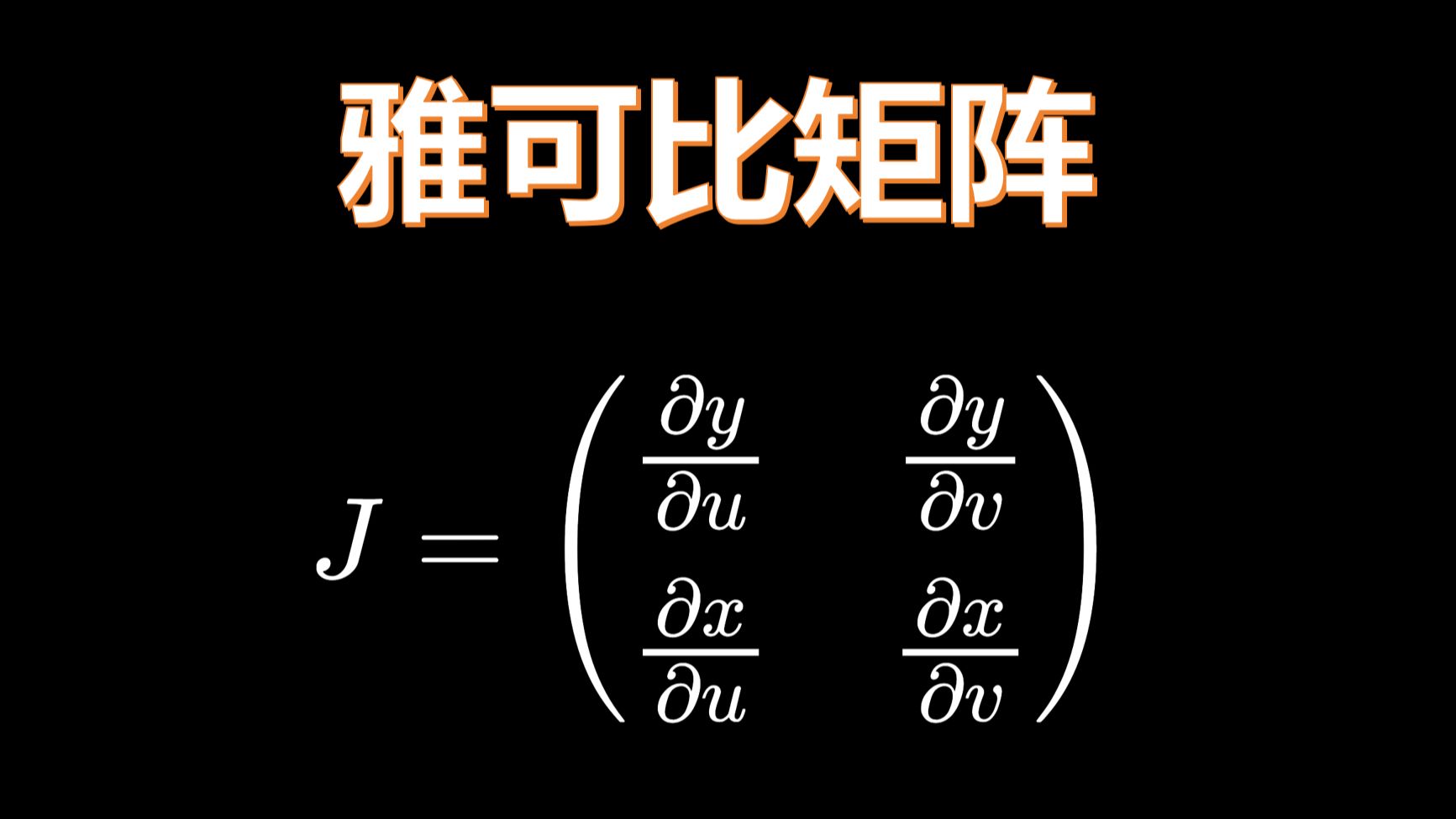 Bilibili18:45.61200000000008