Reviewed learning material · Video analysis · EnglishRead the full overview
This 180-second lecture segment introduces feature scaling in machine learning by explaining why raw features often differ in unit and magnitude. The speaker situates normalization and standardization within feature engineering, defines independent and dependent features in supervised learning, and uses the example “25 years” to separate magnitude from unit. He then argues that datasets with features such as age, weight, and height measured in different ways should be scaled before modeling, naming normalization and standardization as the two common techniques. The clip ends just as he begins defining normalization, so no formulas or full contrast are provided.
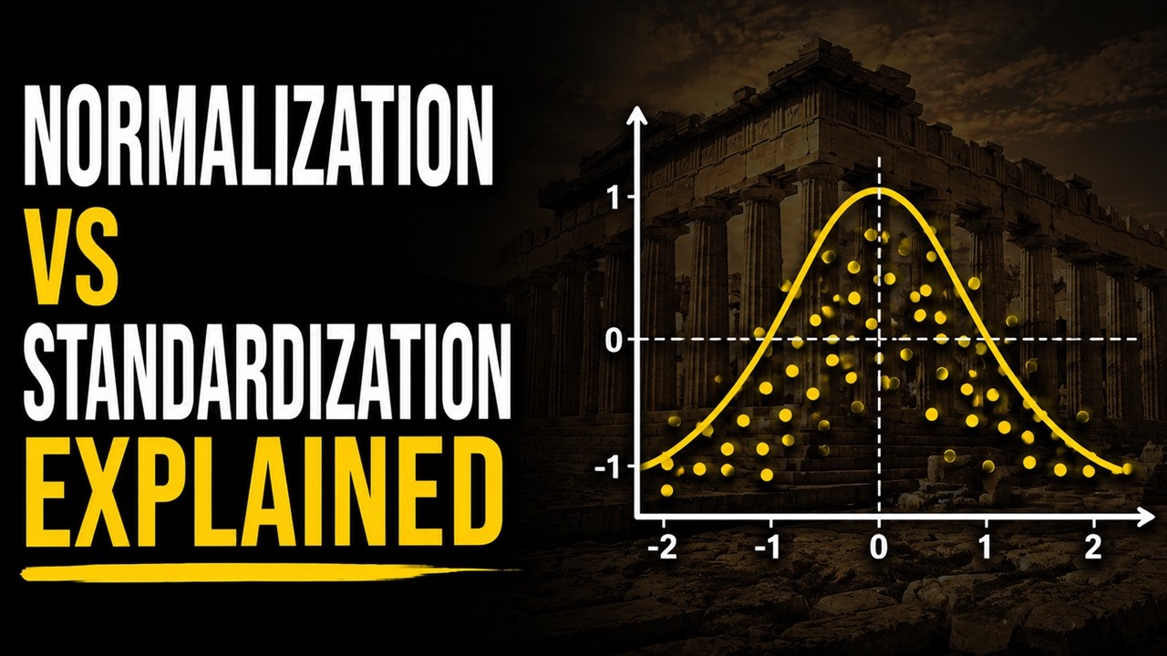
This video segment introduces the concepts of normalization and standardization in feature scaling. The speaker defines normalization as scaling features to a range between 0 and 1, and standardization as scaling features to follow a standard normal distribution (mean 0, standard deviation 1). The segment then transitions to a practical demonstration in a Jupyter Notebook, showing the mathematical formula for min-max normalization and implementing it using the MinMaxScaler class from the scikit-learn library on a sample wine dataset.
This 180-second clip teaches two feature-scaling methods on a small wine dataset in a Jupyter notebook. It first shows raw columns Alcohol and Malic with different magnitudes, then demonstrates MinMaxScaler and displays the formula X_norm=(X-X_min)/(X_max-X_min), explaining that each feature is scaled into [0,1]. It next introduces standardization (z-score normalization) with z=(x-mu)/sigma, stating that each feature is transformed to mean 0 and standard deviation 1, and demonstrates StandardScaler in scikit-learn. A hand-drawn bell curve is used as an intuition aid for the standardized distribution.
This 180-second clip combines a short Jupyter Notebook demonstration of `MinMaxScaler` with a spoken comparison of standardization and normalization. The speaker argues that feature scaling matters for algorithms involving Euclidean distance or gradient descent, naming KNN, K-means, linear regression, logistic regression, ANN, and CNN, while saying tree-based models such as decision trees, random forests, and XGBoost usually do not need scaling. He defines standardization as producing mean 0 and standard deviation 1, and min-max normalization as mapping values into [0,1], especially for image and neural-network inputs.
This 51-second clip is the closing portion of a talk on feature scaling. The speaker says that, in his experience, standardization performs well for most machine learning scenarios, then summarizes that the lesson covered the basic difference between standardization and normalization and was also explained with code. No formulas, derivations, examples, or on-screen mathematics appear in this segment. The remainder is non-mathematical outro content about career advice, a linked channel, subscribing, and saying goodbye.
Use the learning inspector for key ideas and moments, or open the reading tabs for the complete notes.
Generated from the video's visuals and explanation; not verbatim speech.
The segment opens as a spoken introduction to a machine-learning preprocessing topic. The presenter states that the video will explain the basic difference between normalization and standardization, and he places both inside the broader subject of feature scaling, which he calls an integral part of feature engineering.
He then narrows the scope of the lesson: not every algorithm needs feature scaling. This functions as a caution against treating scaling as universal. He also previews later practical material, saying he will discuss when to prefer one technique over another and will eventually demonstrate the ideas with code on a small Kaggle dataset.
To motivate the need for scaling, the speaker shifts to a supervised-learning data workflow. First data are collected; then the dataset contains many features, including independent features and a dependent feature. In this setting, the independent features are used to predict the dependent feature.
Next he identifies two properties that every feature can have: unit and magnitude. These are not introduced with symbols or formulas; instead, they are explained verbally through a concrete person-related dataset containing age, weight, and height.
Using age as the example, he says the unit is the number of years measured from the date of birth. He then isolates the numerical part of a sample value, “25 years,” and explains that 25 is the magnitude while years is the unit. This gives the viewer a simple decomposition of a raw feature value into a number plus a measurement convention.
From that single-feature example, he generalizes to whole datasets. If a dataset has many features, those features will usually be computed using different units and different magnitudes. He reinforces the point with height, noting that it may be recorded in feet or inches. The underlying message is that raw columns are not automatically comparable on the same numerical footing.
This comparison problem becomes the justification for feature scaling. The speaker says it is very necessary, for a machine-learning algorithm, to scale the provided data down into some common scale. He names the two most common techniques for doing this: normalization and standardization.
At the end of the clip, he begins the next step by starting a simple definition of normalization, saying that normalization helps you to scale down your ... The sentence is cut off, so the segment establishes the motivation for scaling but does not yet deliver the full mathematical definition, formula, or contrast with standardization.
The video begins with a verbal definition of normalization, describing it as a process to scale feature values into the interval [0, 1].
Next, standardization is defined as scaling features according to the standard normal distribution, characterized by a mean of 0 and a standard deviation of 1.
The speaker highlights this distinction in target ranges/distributions as the fundamental difference between the two techniques.
The scene shifts to a Jupyter Notebook displaying the mathematical formula for min-max normalization: Xnorm=Xmax−XminX−Xmin.
A practical example follows, showing Python code using pandas to load a subset of the 'wine_data.csv' dataset, selecting the first three columns, renaming them to 'Class', 'Alcohol', and 'Malic', and displaying the first five rows.
Finally, the implementation of normalization is demonstrated using scikit-learn. The code imports `MinMaxScaler`, creates an instance, and applies the `fit_transform` method specifically to the 'Alcohol' and 'Malic' columns of the DataFrame, resulting in scaled values between 0 and 1.
The clip opens on a Jupyter notebook showing the first rows of a wine dataset with columns `Class`, `Alcohol`, and `Malic`. The visible numeric values already differ in size: `Alcohol` is around 13–14, while `Malic` is around 1.7–2.6. The speaker uses this contrast to motivate feature scaling, saying the columns are measured on different units and magnitudes and therefore should be brought onto a comparable scale.
The notebook then shows the min-max workflow in code: `from sklearn.preprocessing import MinMaxScaler`, `scaling=MinMaxScaler()`, and `scaling.fit_transform(df[['Alcohol','Malic']])`. As the output array is scrolled, the speaker points out that the transformed values now lie between 0 and 1, and he highlights entries such as `1.` and `0.5` as evidence of the bounded rescaling.
A Markdown section formalizes the method with the title `Normalization (min-max Normalization)` and the formula Xnorm=Xmax−XminX−Xmin. The explanation is that each feature is handled separately: subtract its own minimum, divide by its own range, and thereby map that feature’s full observed span onto [0,1].
The lesson then switches to the second method, `Standardization(Z-Score Normalization)`. The displayed formula is z=σx−μ, and the accompanying text says the transformed feature should have the properties of a standard normal distribution with mean 0 and standard deviation 1. Conceptually, subtracting μ centers the data at zero, and dividing by σ rescales the spread to unit standard deviation.
The corresponding scikit-learn implementation appears next: `from sklearn.preprocessing import StandardScaler`, `scaling=StandardScaler()`, and `scaling.fit_transform(df[['Alcohol','Malic']])`. The output in `Out[11]` contains both positive and negative numbers, such as `1.51861254` and `-0.5622498`, visually distinguishing standardization from the earlier 0-to-1 normalization.
To build intuition, the presenter sketches a blue bell curve over the notebook while describing a standardized variable as centered at `0`, with successive standard-deviation marks `1, 2, 3` to the right. This drawing is illustrative rather than a computed plot, but it reinforces the idea of centering and unit spacing after z-score transformation.
In the closing seconds, the notebook scrolls back through both sections, leaving the comparison explicit: min-max normalization uses feature minima and maxima to force values into [0,1], while standardization uses the feature mean and standard deviation to produce zero-mean, unit-variance scores. The speaker ends by naming `StandardScaler` and `MinMaxScaler` as the commonly used tools for these tasks.
The clip opens on a static Jupyter Notebook showing three relevant lines: `from sklearn.preprocessing import MinMaxScaler`, `scaling = MinMaxScaler()`, and `scaling.fit_transform(df[['Alcohol', 'Malic']])`. The output below begins with pairs such as `[0.84210526, 0.1916996]` and includes a row starting with `1.`. This visual establishes min-max scaling as a concrete preprocessing step before the lecture turns to the broader question of when to use it.
After the cut to the speaker, the central question becomes: when should one use standardization and when should one use normalization? The answer given is algorithm-dependent rather than universal. The speaker first identifies models involving Euclidean distance, then models trained with gradient descent, as the main families where scaling is important.
Gradient descent is described informally as moving along a parabola-like curve toward a global minimum. In the speaker’s account, scaling the input values helps the optimizer reach that minimum more quickly. This is not presented as a formal convergence theorem in the clip, but as an intuitive engineering rationale for preprocessing.
From that rationale, the lecture names specific algorithms that should use scaling: KNN, K-means clustering, linear regression, logistic regression, artificial neural networks, and convolutional neural networks. The common thread is either distance sensitivity or iterative optimization, both of which can be distorted by unequal feature magnitudes.
The next contrast is with tree-based learners. Decision trees, random forests, XGBoost, and related bagging or boosting methods are said not to require scaling. The reason given is that a tree splits on feature conditions, so whether a feature is numerically large or small does not materially change the branching structure.
The final section compares the two scaling techniques directly. Standardization is defined by its target statistics: mean 0 and standard deviation 1. Min-max normalization is defined by its target interval: values mapped into [0,1]. The speaker adds an experience-based preference, saying standardization worked better for him in many use cases, but immediately qualifies that this does not make min-max scaling bad.
The clip closes by tying min-max scaling to neural networks and image data. Images are described as having pixel values from 0 to 255, and the speaker says these are commonly rescaled to [0,1]. He extends the same logic to ANN and CNN inputs in frameworks such as TensorFlow and Keras, arguing that bounded 0-to-1 inputs help the network learn weights more quickly.
The clip opens mid-thought with the speaker finishing a point about when to use a method, then giving a practical heuristic: for many machine learning scenarios, he has found standardization to perform well. He immediately qualifies this as experience-based advice rather than a formal theorem.
He then closes the mathematical topic by stating that the lesson has covered the basic difference between standardization and normalization, and that he also explained it using code. In this excerpt, however, neither the definitions nor the code are shown again.
After that, the content shifts away from mathematics into channel promotion and career guidance. He mentions a linked resource for data-science career transition advice, asks viewers to subscribe, and ends with a brief farewell.
Knowledge cards
01
Feature scaling in machine learning
This clip introduces feature scaling as a feature-engineering step relevant to machine learning. The speaker says normalization and standardization are important topics within feature scaling and frames the lesson around why scaling is needed and when different algorithms may call for different treatments.
02
Not every algorithm needs feature scaling
The presenter explicitly warns that feature scaling is not necessary for each and every algorithm. In this segment, that point is announced but not yet developed into specific algorithm examples.
03
Independent and dependent features
In the supervised-learning setup described here, collected data contain multiple features, including independent features and a dependent feature. The independent features are used to predict the dependent feature.
04
Unit and magnitude of a feature
The speaker says each feature has two important properties: unit and magnitude. Unit is the measurement convention, while magnitude is the numerical value attached to that measurement.
05
Example: 25 years
Using age as an example, the speaker decomposes “25 years” into magnitude and unit. The magnitude is 25, and the unit is years. This example is used to make the abstract distinction concrete.
06
Why raw features differ across a dataset
When a dataset contains many features, those features are often computed using different units and magnitudes. Height is given as an example that may be measured in feet or inches, showing that columns are not inherently on the same scale.
07
Motivation for scaling data
Because feature units and magnitudes vary, the speaker argues that data provided to a machine-learning algorithm should be scaled into some common scale. Normalization and standardization are named as the two most common techniques for doing this.
08
Beginning of normalization definition
The clip ends just as the speaker starts to define normalization, saying that normalization helps you to scale down your ... No complete definition, formula, or comparison with standardization is delivered within this segment.
09
Normalization Definition
A feature scaling technique that transforms values to lie within a specific range, commonly [0, 1].
Xnorm=Xmax−XminX−Xmin
10
Standardization Definition
A feature scaling technique that transforms data to follow a standard normal distribution with mean 0 and standard deviation 1.
11
Normalization vs Standardization
The core difference is the target: normalization aims for a fixed range (e.g., [0,1]), while standardization aims for a specific statistical distribution (mean 0, std 1).
12
MinMaxScaler Implementation
In scikit-learn, min-max normalization is performed by importing MinMaxScaler, instantiating it, and calling fit_transform on the target feature columns.
13
Why feature scaling is needed
The video begins with a raw wine-data table whose `Alcohol` and `Malic` columns have different numerical magnitudes. The speaker argues that when features differ greatly in scale, they should be transformed onto a comparable scale before further analysis.
14
Min-max normalization formula
Min-max normalization rescales each feature independently using its own minimum and maximum. The displayed rule is Xnorm=Xmax−XminX−Xmin, which maps the feature range onto [0,1].
Xnorm=Xmax−XminX−Xmin
15
MinMaxScaler in scikit-learn
The notebook demonstrates the practical workflow: import `MinMaxScaler`, instantiate it, and call `fit_transform` on the selected columns `['Alcohol','Malic']`. The resulting array entries shown on screen lie between 0 and 1.
16
Standardization / z-score formula
Standardization, also called z-score normalization, transforms each feature using its mean and standard deviation: z=σx−μ. The video states that the transformed feature has mean 0 and standard deviation 1.
z=σx−μ
17
StandardScaler in scikit-learn
The second code demonstration imports `StandardScaler`, creates `scaling=StandardScaler()`, and applies `fit_transform(df[['Alcohol','Malic']])`. Unlike min-max output, the displayed standardized values include negative numbers because the data are centered at 0.
18
Normalization vs standardization
The clip contrasts two scaling strategies on the same features. Min-max normalization bounds values in [0,1] using Xmin and Xmax, while standardization recenters and rescales using μ and σ, producing z-scores that may be negative.
19
Bell-curve intuition for standardization
A hand-drawn bell curve is used to visualize the effect of standardization: the center corresponds to mean 0, and equal steps to the right represent one, two, and three standard deviations. The sketch is illustrative, not a formal proof that every transformed feature becomes exactly normal.
20
Notebook example of MinMaxScaler
A scikit-learn example applies `MinMaxScaler` to the DataFrame columns `Alcohol` and `Malic` with `scaling.fit_transform(df[['Alcohol', 'Malic']])`. The displayed output is a numeric array whose visible entries fall roughly between 0 and 1, illustrating min-max normalization in practice.
The lecture says scaling is important for algorithms that rely on Euclidean distance or gradient-based optimization. Examples named in the clip are KNN, K-means clustering, linear regression, logistic regression, artificial neural networks, and convolutional neural networks.
22
Why tree models usually do not need scaling
Decision trees, random forests, XGBoost, and related bagging/boosting methods are described as not requiring feature scaling because their splits are based on feature conditions rather than absolute magnitude. Rescaling a feature does not substantially change where the branches are created.
23
Standardization target statistics
Standardization is defined verbally as transforming a feature so that its mean becomes 0 and its standard deviation becomes 1. The clip states these target properties but does not show the full algebraic formula.
24
Min-max normalization target range
Min-max normalization is defined as rescaling values into the interval from 0 to 1. The speaker recommends this especially for image inputs and neural-network workflows where bounded inputs are desired.
Detailed learning notes
Explore conditions, steps and evidence. Supplementary explanations are labeled separately from content shown in the video.
Symbols · 26
X_{norm}
Clear evidence
Shown in the video
Evidence
Formula
Observation
The notebook displays the formula Xnorm=Xmax−XminX−Xmin under the heading 'Normalization (min-max Normalization)'.
Symbol
X_{norm}
Meaning
Normalized value of a feature after min-max scaling.
Domain
Real numbers in the interval [0, 1]
X
Clear evidence
Shown in the video
Evidence
Formula
Observation
Appears as the numerator term X in the displayed min-max normalization formula.
Symbol
X
Meaning
Original value of a feature before scaling.
Domain
Real numbers
X_{min}
Clear evidence
Shown in the video
Evidence
Formula
Observation
Appears as Xmin in the displayed min-max normalization formula.
Symbol
X_{min}
Meaning
Minimum value of the feature across the dataset.
Domain
Real numbers
X_{max}
Clear evidence
Shown in the video
Evidence
Formula
Observation
Appears as Xmax in the displayed min-max normalization formula.
Symbol
X_{max}
Meaning
Maximum value of the feature across the dataset.
Domain
Real numbers
df
Clear evidence
Shown in the video
Evidence
Formula
Observation
Python code cell shows `df=pd.read_csv(...)` and later `df.head()`.
Symbol
df
Meaning
Pandas DataFrame object holding the loaded wine dataset.
Domain
Pandas DataFrame
scaling
Clear evidence
Shown in the video
Evidence
Formula
Observation
Python code cell shows `scaling=MinMaxScaler()` and `scaling.fit_transform(df[['Alcohol', 'Malic']])`.
Symbol
scaling
Meaning
Instance of the MinMaxScaler class from scikit-learn used to perform normalization.
Domain
sklearn.preprocessing.MinMaxScaler object
Xnorm
Clear evidence
Shown in the video
Evidence
Formula
Observation
Markdown formula shown on screen: X_norm = (X - X_min) / (X_max - X_min).
Symbol
Xnorm
Meaning
Normalized value of a feature after min-max scaling.
Domain
Real-valued feature values; output is scaled into the interval [0, 1] when X_max > X_min.
X
Clear evidence
Shown in the video
Evidence
Formula
Observation
Appears in the displayed min-max formula X_norm = (X - X_min)/(X_max - X_min).
Audio
Observation
Speaker refers to x as the feature data when explaining standardization and scaling.
Symbol
X
Meaning
Original feature value being transformed.
Xmin
Clear evidence
Shown in the video
Evidence
Formula
Observation
Appears as X_min in the displayed min-max formula.
Symbol
Xmin
Meaning
Minimum value of the feature across the dataset.
Xmax
Clear evidence
Shown in the video
Evidence
Formula
Observation
Appears as X_max in the displayed min-max formula.
Symbol
Xmax
Meaning
Maximum value of the feature across the dataset.
z
Clear evidence
Shown in the video
Evidence
Formula
Observation
Markdown formula shown on screen: z = (x - mu)/sigma.
Audio
Observation
Speaker says this is the basic formula for standardization or z-score normalization.
Symbol
z
Meaning
Standardized feature value, also called a z-score.
μ
Clear evidence
Shown in the video
Evidence
Formula
Observation
Appears as μ in the displayed standardization formula.
Audio
Observation
Speaker explicitly identifies mu as mean.
Symbol
μ
Meaning
Mean of the feature distribution.
Knowledge points · 23
Feature scaling as part of feature engineering
Clear evidence
Shown in the video
Evidence
Audio
Observation
The speaker introduces the topic as “the basic difference between normalization and standardization,” then says it is an important topic in feature scaling, which is part of feature engineering.
Definition
Explanation
In this clip, feature scaling is presented as a feature-engineering step used before discussing when to apply normalization or standardization. The speaker frames the lesson around understanding why feature scaling is needed and what distinguishes normalization from standardization.
Formula
Conditions
The discussion is situated in supervised machine learning and feature engineering.
No mathematical formula is shown in this interval.
Independent and dependent features in supervised machine learning
Clear evidence
Shown in the video
Evidence
Audio
Observation
The speaker says that after collecting data there will be many features, including independent features and a dependent feature, and that with the help of the independent feature one tries to predict the dependent feature in supervised machine learning.
Definition
Explanation
The clip defines the data setting for feature scaling: collected data contains multiple features, among them independent features used to predict a dependent feature in supervised machine learning.
Formula
Conditions
Applies to the supervised machine-learning use case described by the speaker.
No notation or equation is provided.
Unit property of a feature
Clear evidence
Shown in the video
Evidence
Audio
Observation
The speaker states that features have two important properties: unit and magnitude.
Audio
Observation
For age, he says the unit is the number of years from the date of birth.
Audio
Observation
In the example “25 years,” he identifies “years” as the unit.
Definition
Explanation
A unit is the measurement convention attached to a feature value. The speaker illustrates this with age measured in years; in the phrase “25 years,” “years” is the unit.
Formula
Conditions
Introduced through verbal examples rather than formal notation.
The example concerns a person-related dataset with age, weight, and height.
Prerequisites
Independent and dependent features in supervised machine learning
Magnitude property of a feature
Clear evidence
Shown in the video
Evidence
Audio
Observation
The speaker states that features have two important properties: unit and magnitude.
Audio
Observation
He explains magnitude as basically the value.
Audio
Observation
In the example “25 years,” he identifies 25 as the magnitude.
Definition
Explanation
Magnitude is the numerical value associated with a feature measurement. In the speaker’s example “25 years,” the magnitude is 25 while the unit is years.
Formula
Conditions
Presented verbally with a concrete numeric example.
No symbolic representation is displayed.
Prerequisites
Independent and dependent features in supervised machine learning
Why feature scaling is needed
Clear evidence
Shown in the video
Evidence
Audio
Observation
The speaker says that if there are many features, they will definitely be computed using different units and magnitudes.
Audio
Observation
He gives height as an example that may be calculated using feet or inches.
Audio
Observation
He concludes that it is very necessary for machine learning algorithms that the data provided should be scaled down into some scale.
Audio
Observation
He names normalization and standardization as the two most common techniques.
Method
Explanation
The clip argues that raw features often differ in units and magnitudes, so machine-learning input data should be transformed onto a common scale. Normalization and standardization are named as the two most common scaling techniques.
Formula
Conditions
Motivated by datasets with multiple features measured in different units or at different magnitudes.
The clip does not yet provide the formulas or precise target ranges for either technique.
Prerequisites
Unit property of a feature
Magnitude property of a feature
Beginning definition of normalization
Approximate timing
Shown in the video
Evidence
Audio
Observation
The speaker begins, “Now if I give you a simple definition of normalization, normalization helps you to scale down your...” and the clip ends before the sentence is completed.
Uncertainties
The full definition of normalization is cut off before completion.
No formula, range, or contrast with standardization is actually delivered within this clip.
Definition
Explanation
Only the opening of the normalization definition is present in this clip. The speaker starts to say that normalization helps scale down the data, but the explanation is incomplete because the segment ends mid-sentence.
Formula
Conditions
The statement is partial and should not be treated as a full definition.
No mathematical expression is shown.
Prerequisites
Why feature scaling is needed
Definition of Normalization (Min-Max Scaling)
Clear evidence
Shown in the video
Evidence
Audio
Observation
Speaker states: 'normalization helps you to scale down your feature between zero to one.'
Formula
Observation
Notebook text reads: 'In this approach we will scale down the values of the features between 0 to 1.'
Definition
Explanation
Normalization, specifically min-max normalization, is a feature scaling technique that transforms the values of a feature to fit within a specified range, typically between 0 and 1.
Formula
Xnorm=Xmax−XminX−Xmin
Conditions
Applicable to numerical features.
Requires the calculation of minimum and maximum values for the feature.
Assumes Xmax=Xmin to avoid division by zero.
Definition of Standardization
Clear evidence
Shown in the video
Evidence
Audio
Observation
Speaker states: 'Standardization will help you to scale down your feature based on standard normal distribution... mean is usually zero and the standard deviation is usually one.'
Uncertainties
The explicit mathematical formula for standardization is not shown or stated in this clip.
Definition
Explanation
Standardization is a feature scaling technique that transforms data to have properties of a standard normal distribution, meaning it centers the data around a mean of 0 with a standard deviation of 1.
Formula
Conditions
Applicable to numerical features.
Relies on the assumption or goal of approximating a normal distribution.
Using MinMaxScaler in Scikit-Learn
Clear evidence
Shown in the video
Evidence
Formula
Observation
Code cells show `from sklearn.preprocessing import MinMaxScaler`, `scaling=MinMaxScaler()`, and `scaling.fit_transform(df[['Alcohol', 'Malic']])`.
Audio
Observation
Speaker explains creating an object of MinMaxScaler and using `fit_transform` passing specific features.
Method
Explanation
To apply min-max normalization in Python using scikit-learn, one imports the MinMaxScaler class, instantiates it, and calls the fit_transform method on the desired subset of features from a DataFrame.
Formula
Conditions
Requires the scikit-learn library.
Input data must be numerical.
Prerequisites
Definition of Normalization (Min-Max Scaling)
Min-max normalization definition
Clear evidence
Shown in the video
Evidence
Formula
Observation
Markdown heading 'Normalization (min-max Normalization)' with text 'In this approach we will scale down the values of the features between 0 to 1.'
Formula
Observation
Displayed formula X_norm = (X - X_min)/(X_max - X_min).
Audio
Observation
Speaker says values are getting scaled down between 0 to 1.
Definition
Explanation
The video defines min-max normalization as a feature-scaling method that maps each feature's values into the interval from 0 to 1 by subtracting the feature minimum and dividing by the feature range.
Formula
Xnorm=Xmax−XminX−Xmin
Conditions
Applied per feature.
Requires a finite minimum and maximum for the feature.
Markdown heading 'Standardization(Z-Score Normalization)' with text stating features are transformed to have properties of a standard normal distribution with mean(mu)=0 and standard deviation(sigma)=1.
Formula
Observation
Displayed formula z = (x - mu)/sigma.
Audio
Observation
Speaker says standardization is also called z-score normalization and gives the formula x minus mu divided by standard deviation.
Definition
Explanation
The video defines standardization as transforming each feature so that it has mean 0 and standard deviation 1, using the z-score formula.
Formula
z=σx−μ
Conditions
Applied per feature.
Uses the feature mean and standard deviation.
Target transformed statistics are mean 0 and standard deviation 1.
Why feature scaling is used
Clear evidence
Shown in the video
Evidence
Diagram
Observation
Out[3] shows Alcohol values around 13.16 to 14.23 and Malic values around 1.71 to 2.59.
Audio
Observation
Speaker says there is a huge difference between these values and that the magnitude is huge, so we should try to scale down between the same scale.
Method
Explanation
The clip motivates scaling by showing that different columns can have very different magnitudes, so raw values may need to be brought onto a comparable scale before modeling.
Formula
Conditions
Most relevant when features have different units or ranges.
The video does not specify which algorithms require scaling.
Claims and conditions · 7
Difference between Normalization and Standardization
Clear evidence
Shown in the video
Evidence
Audio
Observation
Speaker states: 'So this is the basic difference between standardization and normalization.'
Proposition
Statement
The fundamental difference between normalization and standardization lies in their target distributions/ranges: normalization scales features to a fixed range like [0, 1], while standardization scales features to follow a standard normal distribution (mean 0, std dev 1).
Hypotheses
Both are feature scaling techniques applied to numerical data.
Quantifiers
For all numerical datasets where these techniques are applicable.
Min-max normalization maps values into [0,1]
Clear evidence
Shown in the video
Evidence
Audio
Observation
Speaker says the values are getting scaled down between 0 to 1, the maximum value present over here is 1, and the minimum value will be somewhere between 0 and 1.
Diagram
Observation
Out[8] shows transformed values including 1. and 0.5, with no visible values outside [0,1].
Uncertainties
The spoken phrase 'minimum value will be somewhere between 0 and 1' is less precise than the displayed formula, which implies the minimum becomes 0 for each feature.
Proposition
Statement
After applying min-max normalization, the transformed feature values lie between 0 and 1, with the feature maximum mapped to 1.
Hypotheses
The feature has a well-defined minimum and maximum.
The min-max transformation is applied to that feature.
Quantifiers
For each selected feature column.
Standardization targets mean 0 and standard deviation 1
Clear evidence
Shown in the video
Evidence
Formula
Observation
Markdown text says features will be transformed in such a way that it will have the properties of a standard normal distribution with mean(mu)=0 and standard deviation(sigma)=1.
Audio
Observation
Speaker repeats that the mean will be 0 and standard deviation will be 1 for whichever feature is transformed.
Uncertainties
The video says 'properties of a standard normal distribution'; it does not prove that the resulting distribution is exactly normal for arbitrary data.
Proposition
Statement
Standardization transforms each feature so that its mean is 0 and its standard deviation is 1.
Hypotheses
The feature has a defined mean and nonzero standard deviation.
The z-score transformation is applied feature-wise.
Quantifiers
For each selected feature column.
Scaling formulas are applied independently to each feature
Clear evidence
Shown in the video
Evidence
Audio
Observation
Speaker says the formula that I have actually shown you will get applied to each and every feature.
Proposition
Statement
The scaling formula is applied separately to each feature column.
Hypotheses
Multiple feature columns are present.
Each column is treated as a separate feature.
Quantifiers
For every feature in the selected set.
Speaker’s description of gradient descent
Clear evidence
Shown in the video
Evidence
Audio
Observation
“Gradient descent basically means the parabola curve where you need to find the best minimal point or global minima point.”
Uncertainties
This is a simplified verbal description; the clip does not state assumptions such as convexity or differentiability.
Proposition
Statement
The speaker describes gradient descent as searching along a parabola-like curve to reach the global minimum quickly, and says scaling helps retrieve that point faster.
Hypotheses
The optimization problem is presented informally as having a minima to find.
Feature values can be scaled before optimization.
Quantifiers
Informal universal claim over the algorithms discussed by the speaker.
Empirical preference for standardization
Clear evidence
Shown in the video
Evidence
Audio
Observation
“based on my experience … for many of the use cases where I have actually used standardization … it has basically performed better than the min max scaler.”
Uncertainties
This is an anecdotal experience claim, not a theorem or experimentally established result in the clip.
Conjecture
Statement
The speaker claims that in many of his own use cases, standardization performed better than min-max normalization.
Hypotheses
Comparison is based on the speaker’s personal experience rather than a controlled study shown in the clip.
Quantifiers
Restricted to “many of the use cases” encountered by the speaker.
Neural networks and 0-to-1 inputs
Clear evidence
Shown in the video
Evidence
Audio
Observation
“for most of the deep learning techniques where you're using convolutional neural networks … and artificial neural network, you basically perform min max scaler because you need to scale down your values between 0 to 1.”
Audio
Observation
“libraries like TensorFlow and Keras definitely they will accept inputs between 0 to 1 which will help them to learn the weights quickly.”
Uncertainties
The clip does not provide a formal proof or citation for the library-behavior claim.
Proposition
Statement
The speaker asserts that ANN/CNN workflows commonly use min-max scaling to place inputs in [0,1], and that this helps networks learn weights more quickly.
Hypotheses
Inputs are numerical features or image pixel values.
The model is an artificial or convolutional neural network trained with gradient-based optimization.
Quantifiers
Stated broadly for “most of the deep learning techniques” in the speaker’s framing.
Derivations and proofs · 4
Why min-max output lies in [0,1]
Clear evidence
Derived from the video
Evidence
Formula
Observation
Displayed formula X_norm = (X - X_min)/(X_max - X_min).
Diagram
Observation
Out[8] shows transformed values including 1. and 0.5 within [0,1].
Intuitive argument
Steps
Expression
Xnorm=Xmax−XminX−Xmin
Explanation
Start from the displayed min-max formula.
Justification
Formula shown in the notebook.
Shown in the video
Expression
X=Xmin⇒Xnorm=0
Explanation
Substituting the feature minimum makes the numerator zero.
Justification
Direct substitution into the formula.
Derived from the video
Expression
X=Xmax⇒Xnorm=1
Explanation
Substituting the feature maximum makes numerator and denominator equal.
Justification
Direct substitution into the formula.
Derived from the video
Expression
Xmin≤X≤Xmax⇒0≤Xnorm≤1
Explanation
For any value between the minimum and maximum, the ratio stays between 0 and 1.
Justification
Monotonicity of division by a positive range.
Derived from the video
Conclusion
The min-max transformation maps the feature range [X_min, X_max] onto [0,1].
How z-score standardization produces mean 0 and standard deviation 1
Clear evidence
Derived from the video
Evidence
Formula
Observation
Displayed formula z = (x - mu)/sigma.
Audio
Observation
Speaker explains x minus mu is feature data minus mean, divided by standard deviation.
Intuitive argument
Steps
Expression
z=σx−μ
Explanation
Start from the displayed standardization formula.
Justification
Formula shown in the notebook.
Shown in the video
Expression
x−μ
Explanation
Subtracting the mean centers the feature distribution at 0.
Justification
Definition of mean-centering.
Derived from the video
Expression
σx−μ
Explanation
Dividing by the standard deviation rescales the spread so the new standard deviation is 1.
Justification
Standard property of scaling by a constant factor.
Derived from the video
Conclusion
The z-score transform first centers the data at 0 and then rescales it to unit standard deviation.
Why scaling is recommended for some algorithms
Clear evidence
Shown in the video
Evidence
Audio
Observation
The speaker moves from Euclidean distance and gradient descent to examples such as KNN, K-means, linear regression, logistic regression, ANN, and CNN.
Uncertainties
The reasoning is verbal and intuitive rather than formal.
Intuitive argument
Steps
Expression
Explanation
Identify model families whose behavior depends on feature magnitude, especially distance computations.
Justification
Directly stated by the speaker: algorithms “which involves Euclidean distance.”
Shown in the video
Expression
Explanation
Identify model families trained by iterative optimization toward a minimum.
Justification
Directly stated by the speaker: deep learning techniques “where gradient descent is basically involved.”
Shown in the video
Expression
Explanation
Argue that scaling helps reach the minimum more quickly.
Justification
Speaker’s intuitive explanation linking scaled values to faster retrieval of the minima point.
Shown in the video
Expression
Explanation
List concrete examples needing scaling: KNN, K-means clustering, linear regression, logistic regression, ANN, CNN.
Justification
Named explicitly in the audio.
Shown in the video
Conclusion
Feature scaling is presented as necessary for distance-based and gradient-based learners, but unnecessary for tree-based learners.
Why tree models do not need scaling
Clear evidence
Shown in the video
Evidence
Audio
Observation
“Because at the end of the day you are just creating a decision tree … decision tree is basically divided based on the features.”
Uncertainties
The clip gives only a high-level rationale, not a formal invariance proof.
Intuitive argument
Steps
Expression
Explanation
State that decision-tree methods partition data using feature conditions.
Justification
Directly stated in the audio.
Shown in the video
Expression
Explanation
Observe that changing a feature from large to small values does not substantially alter the branching logic under such conditions.
Justification
Speaker’s informal explanation: “If you keep the value high or if you keep the values small, it won't affect that much.”
Shown in the video
Expression
Explanation
Extend the same reasoning to random forest, XGBoost, bagging, and boosting built on decision trees.
Justification
Explicitly grouped by the speaker with decision-tree methods.
Shown in the video
Conclusion
According to the lecture, tree-based models do not require feature scaling because their splits are condition-based rather than magnitude-sensitive.
Worked examples · 7
Age example distinguishing magnitude and unit
Clear evidence
Shown in the video
Evidence
Audio
Observation
The speaker says he has collected data about a person such as age, weight, and height.
Audio
Observation
He uses the example “25 years,” explaining that 25 is the magnitude and years is the unit.
Problem
Explain how a single feature value can be decomposed into magnitude and unit using age as an example.
Given
A person-related dataset includes features such as age, weight, and height.
One observed age value is stated as 25 years.
Goal
Identify which part of “25 years” is the magnitude and which part is the unit.
Steps
Expression
Explanation
The speaker selects age as a concrete feature from a person-related dataset.
Justification
Stated directly in the audio.
Shown in the video
Expression
Explanation
He describes the unit of age as the number of years from the date of birth.
Justification
Stated directly in the audio.
Shown in the video
Expression
Explanation
For the value “25 years,” he separates the numerical part 25 from the measurement word years.
Justification
Stated directly in the audio.
Shown in the video
Expression
Explanation
He labels 25 as the magnitude and years as the unit.
Justification
Stated directly in the audio.
Shown in the video
Answer
In “25 years,” the magnitude is 25 and the unit is years.
Verification
The example matches the speaker’s explicit verbal decomposition of the phrase into value and unit.
Height example showing unit variation across features
Clear evidence
Shown in the video
Evidence
Audio
Observation
The speaker says that if there are many features, they will be computed using different units and magnitudes.
Audio
Observation
He gives height as an example that may be calculated using feet or inches.
Problem
Show why different features in the same dataset may not share the same unit or magnitude.
Given
A dataset contains multiple features.
Height is one such feature.
Goal
Demonstrate that feature units can vary even within one dataset.
Steps
Expression
Explanation
The speaker generalizes from the age example to datasets with many features.
Justification
Stated directly in the audio.
Shown in the video
Expression
Explanation
He notes that these features will be computed using different units and magnitudes.
Justification
Stated directly in the audio.
Shown in the video
Expression
Explanation
He uses height as a specific example, saying it may be measured in feet or inches.
Justification
Stated directly in the audio.
Shown in the video
Expression
Explanation
This supports the claim that raw feature scales are not inherently aligned across variables.
Justification
Derived from the speaker’s example and conclusion.
Derived from the video
Answer
Height can be represented in feet or inches, illustrating that different features may carry different units and magnitudes.
Verification
The example is consistent with the speaker’s stated motivation for scaling data before machine learning.
Loading and Inspecting Wine Dataset
Clear evidence
Shown in the video
Evidence
Formula
Observation
Code: `df=pd.read_csv('https://raw.githubusercontent.com/rasbt/pattern_classification/master/data/wine_data.csv', header=None, usecols=[0,1,2])` followed by column renaming and `df.head()` output showing columns Class, Alcohol, Malic.
Audio
Observation
Speaker describes reading the CSV, selecting three columns, renaming them, and viewing the top five records.
Problem
Load a subset of the wine dataset and inspect its initial structure.
Given
URL to wine_data.csv
Select first three columns (indices 0, 1, 2)
Rename columns to 'Class', 'Alcohol', 'Malic'
Goal
Display the first five rows of the processed DataFrame.
Steps
Expression
df=pd.readcsv(′...′,header=None,usecols=[0,1,2])
Explanation
Read the CSV file without headers and select only the first three columns.
Justification
Pandas read_csv function usage.
Shown in the video
Expression
df.columns=[′Class′,′Alcohol′,′Malic′]
Explanation
Assign new names to the selected columns.
Justification
Direct assignment to DataFrame columns attribute.
Shown in the video
Expression
df.head()
Explanation
Display the first five rows of the DataFrame.
Justification
Pandas head method default behavior.
Shown in the video
Answer
A table showing 5 rows with columns Class, Alcohol, and Malic containing raw numerical data.
Verification
Visual inspection of the Out[3] cell output matches the described steps.
Applying Min-Max Normalization to Wine Features
Clear evidence
Shown in the video
Evidence
Formula
Observation
Code: `from sklearn.preprocessing import MinMaxScaler`, `scaling=MinMaxScaler()`, `scaling.fit_transform(df[['Alcohol', 'Malic']])`. Output shows arrays of floats between 0 and 1.
Audio
Observation
Speaker explains importing MinMaxScaler, creating an instance, and applying fit_transform to the 'Alcohol' and 'Malic' columns.
Uncertainties
The full output array is truncated in the view; only the beginning is visible.
Problem
Normalize the 'Alcohol' and 'Malic' features of the wine dataset to the range [0, 1].
Given
DataFrame df containing 'Alcohol' and 'Malic' columns
MinMaxScaler from sklearn.preprocessing
Goal
Transform the specified features using min-max scaling.
The original untransformed column values are not visible in this clip, so the exact min and max used by the scaler cannot be verified from the shown output alone.
Problem
Apply min-max scaling to two DataFrame columns in scikit-learn and inspect the transformed output.
Given
A DataFrame `df` exists.
Two selected columns are `Alcohol` and `Malic`.
`MinMaxScaler` is imported from `sklearn.preprocessing`.
Goal
Produce scaled numeric values for the selected columns.
Read the displayed transformed array as the output of the scaling step.
Justification
Visible in the notebook output.
Shown in the video
Answer
The selected columns are transformed into a numeric array whose visible entries lie approximately within 0 to 1.
Verification
Visual check of the output array shows values such as 0.84210526, 0.1916996, and 1.0, consistent with the speaker’s later statement that min-max scaling maps values into [0,1].
Visual events · 11
Lecture-style visual presentation without mathematical graphics
Clear evidence
Shown in the video
Evidence
Diagram
Observation
The entire clip shows a man in a bright pink polo shirt speaking directly to camera against a plain light wall with a whiteboard visible on the right side.
Animation
Observation
He repeatedly gestures with both hands while explaining concepts; no formulas, charts, slides, or written equations appear on screen.
Objects
Presenter in a bright pink polo shirt
Plain light-colored wall
Whiteboard on the right side
Hand gestures
Changes
The presenter changes hand positions and facial expressions while speaking.
No on-screen mathematical content changes because none is displayed.
Invariants
The camera framing remains a medium shot throughout.
No formulas, graphs, tables, or code are shown during the clip.
Interpretation
The mathematical content is conveyed entirely through speech and gesture rather than through visual notation or diagrams.
Jupyter Notebook Navigation
Clear evidence
Shown in the video
Evidence
Animation
Observation
The screen recording scrolls down through a Jupyter Notebook interface, revealing markdown text, formulas, code cells, and output tables/arrays sequentially.
Objects
Markdown headers
LaTeX formula
Python code cells
Dataframe output table
Numpy array output
Changes
Scroll position moves downwards
Different sections of the notebook become visible
Invariants
The content of the notebook remains static during scrolling
Interpretation
Demonstrates the workflow of presenting theory alongside practical code implementation in a computational environment.
Raw feature table before scaling
Clear evidence
Shown in the video
Evidence
Diagram
Observation
Notebook shows Out[3] table with columns Class, Alcohol, Malic and first five rows.
Audio
Observation
Speaker points out that alcohol and malic are noted based on various units and magnitudes and says there is a huge difference.
Objects
DataFrame Out[3]
Columns Class, Alcohol, Malic
Numeric rows 0 through 4
Changes
Mouse highlights different rows while the speaker discusses differing magnitudes.
Invariants
The raw values remain unchanged during this interval.
Only two numeric feature columns are discussed for scaling.
Interpretation
The table visually establishes that the selected features have different numerical ranges, motivating feature scaling.
Scrolling through min-max transformed output
Clear evidence
Shown in the video
Evidence
Diagram
Observation
Code cell In[8] calls scaling.fit_transform(df[['Alcohol','Malic']]) and Out[8] displays a long array of decimal values.
Audio
Observation
Speaker says all the values are getting scaled down between 0 to 1 and points out the maximum is 1.
Uncertainties
Not every row of the output array is readable at once because the user scrolls.
Objects
Out[8] array output
Values such as 0.84210526, 0.1916996, 1., 0.5
Changes
The output area is scrolled to reveal more transformed rows.
Specific values like 1. and 0.5 become visible.
Invariants
All visible transformed values remain within [0,1].
The transformation is applied to the two selected feature columns.
Interpretation
The visual output demonstrates the effect of min-max normalization on the selected features.
Min-max formula displayed in Markdown
Clear evidence
Shown in the video
Evidence
Diagram
Observation
Markdown section titled 'Normalization (min-max Normalization)' appears with explanatory sentence and formula.
Objects
Heading 'Normalization (min-max Normalization)'
Sentence about scaling down values between 0 to 1
Formula X_norm = (X - X_min)/(X_max - X_min)
Changes
The notebook view shifts upward to reveal the Markdown explanation.
Invariants
The formula remains static while the speaker explains it.
Interpretation
This segment supplies the formal definition behind the previously shown MinMaxScaler output.
Standardization formula displayed in Markdown
Clear evidence
Shown in the video
Evidence
Diagram
Observation
Markdown section titled 'Standardization(Z-Score Normalization)' appears with text about mean(mu)=0 and standard deviation(sigma)=1 and formula z = (x - mu)/sigma.
Objects
Heading 'Standardization(Z-Score Normalization)'
Explanatory sentence about standard normal properties
Formula z = (x - mu)/sigma
Changes
The notebook view shifts to the standardization section.
Invariants
The formula and target statistics remain fixed during the explanation.
Interpretation
This segment introduces the mathematical rule for z-score standardization before the code demonstration.
Scrolling through standardized output
Clear evidence
Shown in the video
Evidence
Diagram
Observation
Code cells In[9]-In[11] and Out[11] show StandardScaler usage and transformed array values including negatives.
Uncertainties
Exact full extent of the dataset is not visible.
Objects
Out[11] array output
Values such as 1.51861254, -0.5622498, -1.25345042
Changes
The output area is scrolled to reveal many standardized rows.
Invariants
The selected columns remain ['Alcohol','Malic'].
The transformation is based on the displayed z-score formula.
Interpretation
The output visually contrasts with min-max scaling by showing both positive and negative centered values.
Hand-drawn bell curve illustrating standardization
Clear evidence
Shown in the video
Evidence
Animation
Observation
A blue bell-shaped curve is drawn over the notebook output area.
Audio
Observation
Speaker says if it is getting converted into standard normal distribution it will be converted like this into a bell curve, with mean over here as 0 and each standard deviation to the right as 1, 2, 3.
Uncertainties
The drawing is schematic and not an actual plotted histogram of the dataset.
Objects
Blue bell-shaped curve
Implied horizontal axis
Spoken labels 0, 1, 2, 3
Changes
A curve is sketched freehand over the notebook.
The speaker verbally marks the center as 0 and steps to the right as 1, 2, 3.
Invariants
The sketch is illustrative rather than a computed plot.
The intended invariant is centering at 0 with unit spacing for standard deviations.
Interpretation
The drawing provides an intuitive picture of a standardized variable as a symmetric distribution centered at 0 with standard-deviation units marked along the axis.
Static notebook view of scaling code
Clear evidence
Shown in the video
Evidence
Diagram
Observation
A Jupyter Notebook interface fills the screen with code cells and an output array.
Formula
Observation
The code and output remain static during this interval.
Objects
Jupyter Notebook window
code cells
output array
mouse cursor
Changes
No scrolling or code execution occurs within the visible interval.
Invariants
The same three code lines and the beginning of the output array stay on screen.
Interpretation
The visual establishes the practical implementation context for min-max normalization before the lecture switches to conceptual discussion.
Lecture gestures accompanying verbal explanation
Clear evidence
Shown in the video
Evidence
Animation
Observation
The speaker repeatedly raises both hands, points, opens palms, and makes small pinching motions while talking.
Diagram
Observation
At about 00:00:33 he traces a curved motion in the air while discussing gradient descent and minima.
Objects
male speaker
white wall
whiteboard edge
hand gestures
Changes
Camera cuts from notebook to speaker at 00:00:15.
Hand motions intensify when contrasting algorithms and explaining scaling choices.
Invariants
No formulas, plots, or diagrams are drawn on screen during the talking-head portion.
Interpretation
The gestures function as emphasis only; the mathematical content is carried by speech rather than by on-screen notation.
Presenter-only closing shot
Clear evidence
Shown in the video
Evidence
Diagram
Observation
The entire clip shows a man speaking directly to camera against a plain wall, using hand gestures; no formulas, plots, tables, or code are visible.
Objects
single presenter
plain wall background
hand gestures
Changes
The speaker continues talking and gesturing throughout the clip.
Invariants
No mathematical notation appears on screen.
No code window or example output is shown in this segment.
Interpretation
The visual track supports a spoken wrap-up and recommendation segment rather than a worked mathematical demonstration.
Misconceptions · 6
Feature scaling is not universally required for every algorithm
Clear evidence
Shown in the video
Evidence
Audio
Observation
The speaker says it is not necessary to apply feature scaling for each and every algorithm, and that the video will discuss when to prefer normalization or standardization and for which algorithms feature scaling suits.
Uncertainties
The clip announces this distinction but does not yet provide the actual algorithm-by-algorithm guidance.
Misconception
One might assume that every machine-learning algorithm requires feature scaling.
Clarification
The speaker explicitly warns that feature scaling is not necessary for each and every algorithm, although this clip only previews that later discussion without giving the detailed cases.
Confusing bounded rescaling with centering/scaling
Clear evidence
Shown in the video
Evidence
Diagram
Observation
Min-max output in Out[8] stays in [0,1], while standardization output in Out[11] includes negative values.
Audio
Observation
Speaker distinguishes min-max scaling between 0 to 1 from standardization with mean 0 and standard deviation 1.
Misconception
One might think all feature scaling methods force values into the same fixed interval.
Clarification
The clip shows two different rules: min-max normalization maps each feature into [0,1], whereas standardization recenters and rescales to mean 0 and standard deviation 1, allowing negative values.
Standardization does not guarantee normality
Approximate timing
Supplementary explanation
Evidence
Formula
Observation
Markdown text says transformed features will have the properties of a standard normal distribution with mean(mu)=0 and standard deviation(sigma)=1.
Audio
Observation
Speaker repeats the standard-normal wording and later draws a bell curve.
Uncertainties
This clarification is added by the analyst; the video itself does not discuss non-normal input distributions.
Misconception
Standardization makes any feature follow a normal distribution.
Clarification
Editorial note: the formula guarantees mean 0 and standard deviation 1, but it does not transform an arbitrary distribution into an exactly normal one. The video's bell-curve sketch is only an illustration.
Assuming every machine-learning model needs feature scaling
Clear evidence
Shown in the video
Evidence
Audio
Observation
The speaker explicitly contrasts tree-based models with distance- and gradient-based models to say scaling is not needed for the former.
Misconception
One might think feature scaling is always required before training any model.
Clarification
The lecture states that decision trees, random forests, XGBoost, and related bagging/boosting methods do not need scaling because their splits are based on feature conditions rather than absolute magnitude.
Treating min-max scaling as inferior overall
Clear evidence
Shown in the video
Evidence
Audio
Observation
“Now it is not like that min max scaler is bad and it should not be used.”
Misconception
After hearing that standardization often worked better for the speaker, one might conclude min-max scaling should be avoided.
Clarification
The speaker immediately adds that min-max scaling is still appropriate for many deep-learning settings, especially when inputs should be bounded between 0 and 1.
Do not treat the recommendation as a universal theorem
Clear evidence
Shown in the video
Evidence
Audio
Observation
The speaker explicitly says the claim that standardization performs well is "completely based on my experience."
Misconception
One might hear "standardization performs well" as a general mathematical fact valid for all machine learning models and datasets.
Clarification
The clip presents it as the speaker's experiential observation for many scenarios, not as a proven statement with stated assumptions or counterexample analysis.
Concept relations · 20
Feature scaling as part of feature engineering → Why feature scaling is needed
Clear evidence
Shown in the video
Evidence
Audio
Observation
The speaker says normalization and standardization are important topics in feature scaling, which is an integral part of feature engineering.
Contains
Explanation
The clip places normalization and standardization inside the broader workflow of feature scaling and feature engineering.
Independent and dependent features in supervised machine learning → Unit property of a feature
Clear evidence
Shown in the video
Evidence
Audio
Observation
After defining independent and dependent features in a supervised-learning dataset, the speaker says those features have two important properties: unit and magnitude.
Contains
Explanation
The discussion of dataset features leads directly into the two properties used to motivate scaling.
Magnitude property of a feature → Why feature scaling is needed
Clear evidence
Shown in the video
Evidence
Audio
Observation
The speaker argues that because many features have different units and magnitudes, it is necessary to scale the data for machine learning algorithms.
Application
Explanation
The property of differing magnitudes is used as a reason to apply feature scaling.
Unit property of a feature → Why feature scaling is needed
Clear evidence
Shown in the video
Evidence
Audio
Observation
The speaker uses varying units such as feet and inches for height to justify scaling data into a common scale.
Application
Explanation
The property of differing units is also used as a reason to apply feature scaling.
Why feature scaling is needed → Beginning definition of normalization
Approximate timing
Shown in the video
Evidence
Audio
Observation
After naming normalization and standardization as the two common techniques, the speaker begins a definition of normalization.
Uncertainties
The definition is incomplete because the clip ends mid-sentence.
Special case
Explanation
Normalization is introduced as one of the two common methods for carrying out the previously motivated feature scaling.
Definition of Normalization (Min-Max Scaling) → Definition of Standardization
Clear evidence
Shown in the video
Evidence
Audio
Observation
Speaker explicitly contrasts the two definitions given just prior.
Contrast
Explanation
Normalization targets a fixed range [0,1], whereas standardization targets a distribution with mean 0 and variance 1.
Definition of Normalization (Min-Max Scaling) → Using MinMaxScaler in Scikit-Learn
Clear evidence
Shown in the video
Evidence
Formula
Observation
The mathematical formula is presented immediately before the code implementing it.
Application
Explanation
The MinMaxScaler class in scikit-learn is the software implementation of the mathematical min-max normalization formula.
Why feature scaling is used → Min-max normalization definition
Clear evidence
Shown in the video
Evidence
Audio
Observation
Speaker first notes huge differences in magnitude, then says we should try to scale down between the same scale and introduces MinMaxScaler.
Diagram
Observation
Raw table Out[3] precedes MinMaxScaler code and output Out[8].
Application
Explanation
The observed difference in feature magnitudes motivates applying min-max normalization.
Why feature scaling is used → Standardization / z-score normalization definition
Clear evidence
Shown in the video
Evidence
Audio
Observation
After discussing differing magnitudes, the speaker moves to standardization as another way to transform features.
Diagram
Observation
The notebook proceeds from raw data to standardization formula and StandardScaler code.
Application
Explanation
The same motivation of putting features on comparable scales leads to the introduction of standardization.
Two Markdown sections display different formulas: X_norm = (X - X_min)/(X_max - X_min) and z = (x - mu)/sigma.
Diagram
Observation
Out[8] shows values in [0,1]; Out[11] shows positive and negative z-scores.
Contrast
Explanation
The clip directly contrasts bounded min-max rescaling with mean-centering and variance-normalizing standardization.
Min-max normalization definition → Using MinMaxScaler in scikit-learn
Clear evidence
Shown in the video
Evidence
Formula
Observation
MinMaxScaler code is shown alongside the min-max Markdown formula.
Application
Explanation
The mathematical definition is implemented in the notebook through MinMaxScaler.fit_transform.
Standardization / z-score normalization definition → Using StandardScaler in scikit-learn
Clear evidence
Shown in the video
Evidence
Formula
Observation
StandardScaler code is shown alongside the z-score Markdown formula.
Application
Explanation
The z-score definition is implemented in the notebook through StandardScaler.fit_transform.
Find an answer · 25
Why do we need feature scaling before feeding data to a machine learning algorithm?
Clear evidence
Shown in the video
Evidence
Audio
Observation
The speaker explains that different features have different units and magnitudes and therefore should be scaled for machine learning.
Knowledge points
Unit property of a feature
Magnitude property of a feature
Why feature scaling is needed
What is the difference between unit and magnitude in a feature value?
Clear evidence
Shown in the video
Evidence
Audio
Observation
The speaker distinguishes magnitude as the value and unit as the measurement convention, using “25 years” as the example.
Knowledge points
Unit property of a feature
Magnitude property of a feature
Age example distinguishing magnitude and unit
Which two common techniques are introduced for feature scaling?
Clear evidence
Shown in the video
Evidence
Audio
Observation
The speaker names normalization and standardization as the two most common techniques used for scaling data.
Knowledge points
Why feature scaling is needed
Does every machine learning algorithm require feature scaling?
Clear evidence
Shown in the video
Evidence
Audio
Observation
The speaker says feature scaling is not necessary for each and every algorithm.
Uncertainties
The clip does not specify which algorithms do or do not require scaling.
Knowledge points
Feature scaling is not universally required for every algorithm
How does the speaker begin defining normalization?
Approximate timing
Shown in the video
Evidence
Audio
Observation
The speaker begins to define normalization but the sentence is cut off before completion.
Uncertainties
The full definition is absent from this clip.
Knowledge points
Beginning definition of normalization
What is the definition of normalization in feature scaling?
Clear evidence
Shown in the video
Evidence
Audio
Observation
Initial definition provided by speaker.
Knowledge points
Definition of Normalization (Min-Max Scaling)
How does standardization differ from normalization?
Clear evidence
Shown in the video
Evidence
Audio
Observation
Speaker defines both and states the difference.
Knowledge points
Definition of Normalization (Min-Max Scaling)
Definition of Standardization
Difference between Normalization and Standardization
What is the mathematical formula for min-max normalization?
Clear evidence
Shown in the video
Evidence
Formula
Observation
Formula clearly displayed in notebook.
Knowledge points
Definition of Normalization (Min-Max Scaling)
How do I use MinMaxScaler in scikit-learn?
Clear evidence
Shown in the video
Evidence
Formula
Observation
Code cells demonstrate usage.
Knowledge points
Using MinMaxScaler in Scikit-Learn
What is the min-max normalization formula and what range does it produce?
Clear evidence
Shown in the video
Evidence
Formula
Observation
Markdown section explicitly defines min-max normalization and shows the formula.
Knowledge points
Min-max normalization definition
Min-max normalization maps values into [0,1]
Why min-max output lies in [0,1]
Why do we need feature scaling when columns have different magnitudes?
Clear evidence
Shown in the video
Evidence
Diagram
Observation
Raw table shows different magnitudes across Alcohol and Malic.
Audio
Observation
Speaker says there is a huge difference and we should scale down between the same scale.
Knowledge points
Why feature scaling is used
How do I apply min-max normalization in scikit-learn?
Clear evidence
Shown in the video
Evidence
Formula
Observation
Code cells show import MinMaxScaler and fit_transform usage.
Knowledge points
Using MinMaxScaler in scikit-learn
Wine dataset min-max scaling example
Coverage and review notes
Covered · Introduction to normalization, standardization, feature scaling, and feature engineering.
Covered · Speaker previews that different algorithms may call for different scaling choices and mentions a later coding example; no new mathematics is developed here.
Covered · Supervised-learning setup with independent and dependent features.
Covered · Definition of unit and magnitude illustrated with age = 25 years.
Covered · Argument that differing units and magnitudes across features motivate scaling; height in feet or inches is used as an example.
Covered · Opening of the normalization definition is present but incomplete because the clip ends mid-sentence.
Covered · Spoken introduction defining normalization and standardization and contrasting them.
Covered · Visual presentation of the min-max normalization formula in a Jupyter Notebook.
Covered · Code demonstration of loading and inspecting the wine dataset.
Covered · Code demonstration of applying MinMaxScaler to specific features.
Covered · Raw wine-data table is shown and the speaker motivates scaling because Alcohol and Malic have different magnitudes.
Covered · MinMaxScaler code and transformed output are shown; speaker states values are scaled between 0 and 1.
Covered · Markdown section displays the min-max formula and the speaker says it is applied to each feature.
Covered · Markdown section introduces standardization / z-score normalization with formula z=(x-mu)/sigma and target mean 0, std 1.
Covered · StandardScaler import, object creation, and fit_transform output are shown; transformed values include negatives.
Covered · A hand-drawn bell curve illustrates the idea of a standardized distribution centered at 0 with unit standard-deviation spacing.
Covered · The notebook scrolls back through both methods while the speaker summarizes that StandardScaler and MinMaxScaler are the popular libraries used for these transformations.
Covered · Static notebook view showing MinMaxScaler import, instantiation, fit_transform on Alcohol and Malic, and output array.
Covered · Talking-head explanation of when scaling is needed, with examples of distance-based, gradient-based, and tree-based algorithms.
Covered · Direct comparison of standardization and min-max normalization, including target statistics, image example, and neural-network use case.
Covered · Spoken practical recommendation about standardization in machine learning.
Covered · Spoken summary that the lesson covered the basic difference between standardization and normalization and included code.
Reviewed English material v1: card/concept_card "Beginning of normalization definition" starting at 2:54 — The clip ends just as the speaker starts to define normalization, saying that normalization helps you to scale down your ... No complete definition, formula, or comparison with standardization is delivered within this segment.
Decision-tree models do not require feature scaling because they split data based on feature conditions (thresholds) rather than absolute magnitudes. Monotonic rescaling of feature values does not change the branching structure or the order of splits.
Conditions: Model is a decision tree or an ensemble of trees (random forest, XGBoost, etc.).; Splitting logic is based on comparing feature values to thresholds.
Feature scaling is needed because raw features often differ in units and magnitudes, making them incomparable. Scaling brings them onto a common scale, which is necessary for many machine learning algorithms to function properly.
Conditions: Dataset contains multiple features with different units or ranges.; The model is sensitive to feature magnitudes (e.g., distance-based or gradient-based).
Import `MinMaxScaler` from `sklearn.preprocessing`, instantiate it, and call `fit_transform` on the selected DataFrame columns. This fits the scaler to the data (learning min/max) and transforms the values to the [0, 1] range.
Conditions: Input data is numerical.; Scikit-learn library is installed.
Import `StandardScaler` from `sklearn.preprocessing`, instantiate it, and call `fit_transform` on the selected DataFrame columns. This transforms the data to have mean 0 and standard deviation 1.
Conditions: Input data is numerical.; Scikit-learn library is installed.
Min-max normalization transforms a feature value X into Xnorm=Xmax−XminX−Xmin, mapping the feature's observed range onto the interval [0,1].
Conditions: Applied per numerical feature.; Requires a finite minimum Xmin and maximum Xmax for the feature.; Assumes Xmax=Xmin to avoid division by zero.
Feature scaling should be used for algorithms that rely on Euclidean distance or gradient-based optimization, such as KNN, K-means, linear regression, logistic regression, and neural networks. It is generally not needed for tree-based models like decision trees, random forests, and XGBoost.
Conditions: Model uses distance metrics or iterative optimization sensitive to feature scale.; Model is not tree-based or an ensemble of trees.
Standardization centers data at the mean (μ), so values below the mean become negative. Min-max normalization shifts and scales data so the minimum becomes 0 and the maximum becomes 1, keeping all values non-negative within [0, 1].