Definite integral as a core calculus idea
The opening names the topic. The full video then develops a curve-area interpretation and writes its notation; it does not give a formal sum-limit definition.
 mathvideo•
Connect a nonnegative curve-area diagram to definite-integral notation, with bilingual notes on bounds, integrand and signed-area conditions.
Connect a nonnegative curve-area diagram to definite-integral notation. Khan Academy sketches f(x), marks a and b, shades the region above the horizontal axis and then writes ∫ from a to b of f(x) dx, explaining its bounds, integrand and integration variable. This complete short lesson teaches the geometric meaning and notation, without a numerical computation, Riemann-sum construction or fundamental-theorem proof. Editorial notes state integrability and nonnegativity for ordinary area, and distinguish general signed accumulation.
Generated from the video's visuals and explanation; not verbatim speech.
Introduce definite integrals alongside derivatives and antiderivatives; the lesson then builds a geometric interpretation.
Begin with areas under curves, using a picture before the notation.
Draw two coordinate systems. The full lesson uses the left graph; the right graph remains unused.
Sketch a positive curve f(x) above the horizontal axis. No explicit numeric function is supplied.
Mark x=a on the left in red and x=b to its right in green, defining the interval boundaries.
Identify the region beneath y=f(x) between the two endpoints; the continuation will shade it and write the integral.
Shade the region below the curve, above the horizontal axis and between x=a and x=b. For ordinary area, use a<b and an integrable, nonnegative f; continuity is sufficient for integrability.
A curved boundary can be handled with integral calculus; this schematic lesson does not compute a numeric area.
Write the integral sign beside the diagram to turn the geometric object into notation.
Add lower bound a, upper bound b, integrand f(x) and dx, which specifies integration with respect to x.
The presenter previews a later explanation through Riemann sums and mentions Leibniz in a brief background comment; no historical derivation or sum construction is shown.
In this nonnegative, integrable case, equals the shaded area. In general the integral is signed accumulation; ordinary area for a sign-changing function uses |f| when integrable.
The opening names the topic. The full video then develops a curve-area interpretation and writes its notation; it does not give a formal sum-limit definition.
Use the pictured nonnegative curve to motivate ordinary area. For a<b and integrable nonnegative f, this area equals its definite integral.
The graph labels f(x) and the left/right endpoints a,b. These mark the region above the horizontal axis; no numeric function or endpoint values are given.
The opening setup identifies the curve and boundaries before notation appears later in the same full video. Riemann sums and numeric computations are outside this lesson.
For a<b and integrable, nonnegative f on [a,b], the integral equals ordinary area beneath the graph. More generally an integral records signed accumulation; ordinary area for sign-changing f uses |f|, when integrable.
a and b are the lower and upper bounds, f(x) is the integrand, and dx specifies the variable x of integration.
The presenter connects the integral sign with Leibniz in a brief comment. This is an attributed video remark, not a historical proof or a verified alternate technical name.
The video previews a future explanation of notation with Riemann sums; it does not construct a sum or take its limit here.
The shaded ordinary area equals the displayed integral for the pictured nonnegative integrable function and ordered endpoints. No numeric area is calculated.
Explore conditions, steps and evidence. Supplementary explanations are labeled separately from content shown in the video.
White handwritten title “Definite Integral” is written at the upper left of a black digital canvas.
The presenter introduces the definite integral as a core calculus topic.
Definite Integral
Title naming the mathematical concept being introduced.
Calculus topic name; no numerical domain is given in this clip.
A vertical white axis with an upward arrowhead is drawn on the left coordinate system.
The presenter labels the vertical coordinate axis.
y
Vertical coordinate axis label for the first Cartesian plane.
Coordinate axis label; no scale or units are shown.
A horizontal white axis with a rightward arrowhead is drawn on the left coordinate system.
The presenter labels the horizontal coordinate axis.
x
Horizontal coordinate axis label for the first Cartesian plane.
Coordinate axis label; no scale or units are shown.
A second vertical white axis with an upward arrowhead is drawn to the right of the first coordinate system.
The presenter labels the vertical coordinate axis.
The second coordinate system remains empty through the end of the clip, so its intended use is not stated here.
y
Vertical coordinate axis label for the second Cartesian plane.
Coordinate axis label; no scale or units are shown.
A second horizontal white axis with a rightward arrowhead is drawn on the right coordinate system.
The presenter labels the horizontal coordinate axis.
The second coordinate system remains empty through the end of the clip, so its intended use is not stated here.
x
Horizontal coordinate axis label for the second Cartesian plane.
Coordinate axis label; no scale or units are shown.
A red wavy curve is drawn above the x-axis on the left coordinate system, then labeled “f(x)” in red near the curve.
The narration identifies the function represented by the red curve.
No explicit formula for f is given; only a schematic graph is shown.
f(x)
Name of the plotted function whose graph is drawn in red.
Function notation; the displayed graph lies above the x-axis on the shown interval, but no formal domain or range is specified.
A red tick mark labeled “a” is placed on the positive x-axis of the left graph, and a red vertical segment is drawn upward from that point toward the curve.
The presenter identifies the left interval boundary.
The exact numerical value of a is not given.
a
Left endpoint of the x-interval under consideration.
Real number used as a lower limit marker on the x-axis; visually placed to the right of the origin and left of b.
A green tick mark labeled “b” is placed farther right on the positive x-axis of the left graph, and a green vertical segment is drawn upward from that point toward the curve.
The presenter identifies the right interval boundary.
The exact numerical value of b is not given.
b
Right endpoint of the x-interval under consideration.
Real number used as an upper limit marker on the x-axis; visually placed to the right of a.
The narration focuses on the region under the function graph.
The previously drawn red curve on the left graph is the object referred to by this equation.
y = f(x)
Equation of the plotted curve whose under-graph area is being introduced.
Cartesian equation relating vertical coordinate y to the function value f(x).
The horizontal axis of the coordinate system on the left is labeled x.
x
Independent variable / horizontal coordinate
Position variable on the real number line
The vertical axis of the coordinate system on the left is labeled y.
y
Dependent variable / vertical coordinate
Vertical coordinate where the function value lies
Next to the red curve, it is written y=f(x).
The narration identifies the function represented by the red curve.
f(x)
Integrand, i.e., the function value of the red curve in the diagram
On the interval [a,b], used to represent the integrand for the area under the curve
The presenter introduces the definite integral as a core calculus topic.
The presenter introduces the definite integral as a core calculus topic.
The title “Definite Integral” is written on screen during this introduction.
The opening introduces the topic before a geometric construction. The same full video then represents a nonnegative-curve area with integral notation, without a formal Riemann-sum definition.
The opening interval is motivation, not a formal definition.
The narration focuses on the region under the function graph.
Two blank Cartesian coordinate systems are drawn, then the left one receives a red curve labeled f(x), a red vertical marker at x=a, and a green vertical marker at x=b.
The narration focuses on the region under the function graph.
The curve is schematic; no numeric formula or area calculation is supplied. Shading and notation follow after this opening interval in the complete video.
The method shown is to represent the problem geometrically: draw coordinate axes, sketch a function y=f(x), mark two x-values a and b, and identify the region under the graph between those markers as the object of interest. This prepares the intuitive basis for the definite integral without yet writing the integral symbolically.
Uses a Cartesian graph.
The function is represented schematically rather than by an explicit formula.
The interval endpoints are marked as x=a and x=b.
a<b and f is integrable on [a,b]; continuity is a sufficient condition.
For this ordinary area interpretation, f is nonnegative on [a,b].
The presenter identifies the region above the horizontal axis and under the curve between the two interval boundaries.
In the left diagram, the region enclosed by the red curve y=f(x), the x-axis, and the vertical lines x=a and x=b is filled with diagonal hatching.
The presenter identifies the region above the horizontal axis and under the curve between the two interval boundaries.
For a<b and integrable, nonnegative f on [a,b], the definite integral equals the area between its graph and the horizontal axis. Continuity suffices for integrability here. In general, the integral is signed accumulation; where f changes sign, ordinary area uses the integral of |f|, when integrable. These conditions and the signed-area distinction are editorial clarification of the pictured positive-curve case.
a<b and f is integrable on [a,b]; continuity is a sufficient condition.
For this ordinary area interpretation, f is nonnegative on [a,b].
The presenter writes the integral notation in stages and connects its parts with the diagram.
On the right, the integral sign ∫ is written step by step, followed by the lower limit a, upper limit b, integrand f(x), and dx.
The presenter writes the integral notation in stages and connects its parts with the diagram.
The video writes the previously described area using the standard notation \int_a^b f(x)\,dx. Here, a is the lower limit, b is the upper limit, f(x) is the integrand, and dx indicates the variable of integration. Each part of the notation corresponds one-to-one with the boundaries and curve in the left diagram.
Used to represent the definite integral from x=a to x=b
The integrand is f(x)
The presenter gives a brief background comment linking the integral sign to Leibniz.
No detailed historical evidence or exact technical-name verification is provided in this lesson.
The presenter briefly links the integral sign with Leibniz and previews a future explanation through sums. This lesson does not give a historical account or a formal sum construction.
The ending identifies the written integral with the shaded area in the pictured case.
The ending identifies the written integral with the shaded area in the pictured case.
On the right, ∫_a^b f(x) dx has been written out, corresponding to the shaded region on the left.
Under the conditions shown in this segment, the shaded area on the left, enclosed by y=f(x), the x-axis, x=a, and x=b, is equal to the value represented by the expression \int_a^b f(x)\,dx on the right.
The region is above the x-axis
The left and right boundaries are x=a and x=b
The upper boundary is the curve y=f(x)
a<b and f is integrable on [a,b]; continuity is a sufficient condition.
For this ordinary area interpretation, f is nonnegative on [a,b].
For the specific curve and interval [a,b] in this example
The narration emphasizes that area problems can include curved boundaries.
The narration emphasizes that area problems can include curved boundaries.
One function of the definite integral is its ability to calculate the area of regions whose boundaries include curves, not limited to conventional area problems with only straight-line boundaries.
The discussed region can be enclosed by a function curve, coordinate axes, and vertical boundaries
a<b and f is integrable on [a,b]; continuity is a sufficient condition.
For this ordinary area interpretation, f is nonnegative on [a,b].
General statement, but this segment only provides one illustrative example
The presenter writes the integral notation in stages and connects its parts with the diagram.
On the right, ∫, a, b, f(x), and dx are written sequentially to form the complete expression.
In the left diagram, a, b, f(x), and the shaded region are visible simultaneously, facilitating the establishment of correspondence.
First, write the integral symbol to indicate the introduction of the definite integral notation.
Introduce the integral notation for the pictured area.
Write a below the integral symbol to represent the left boundary/lower limit.
The lower bound corresponds to the left endpoint.
Write b above the integral symbol to represent the right boundary/upper limit.
The upper bound corresponds to the right endpoint.
Write the integrand f(x), corresponding to the area under the curve y=f(x).
The integrand corresponds to the plotted function.
Finally, add dx to complete the entire definite integral expression.
The final notation specifies the integration variable.
The shaded area on the left is completely translated into the notation \int_a^b f(x)\,dx on the right.
The presenter previews a future explanation using Riemann sums without giving the sum construction here.
This segment does not actually expand on Riemann sum formulas or limit processes; it only previews that the source of the notation will be explained later.
The video first gives the intuitive meaning of the notation \int_a^b f(x)\,dx, then states that its origin will be explained later.
The narrator previews a future connection with Riemann sums, without presenting that construction now.
This segment only establishes the intuitive meaning of the definite integral notation and does not provide a rigorous Riemann sum derivation.
In the left coordinate system, the red curve y=f(x) is drawn, and the region between the curve and the x-axis from x=a to x=b is filled with diagonal hatching.
The presenter identifies the region above the horizontal axis and under the curve between the two interval boundaries.
On the right, \int_a^b f(x)\,dx is written to represent this area.
Given the curve y=f(x) and the x-axis, as well as two vertical boundaries x=a and x=b, express the area of the upper region they enclose.
Function curve y=f(x)
Left boundary x=a
Right boundary x=b
Region is above the x-axis
a<b and f is integrable on [a,b]; continuity is a sufficient condition.
For this ordinary area interpretation, f is nonnegative on [a,b].
Use definite integral notation to represent the area of this shaded region.
First, determine which lines enclose the area from the diagram.
The left diagram clearly marks the curve, two vertical lines, and the x-axis.
The narrator explains that this kind of curved-boundary area is exactly what the definite integral expresses.
With an integrable nonnegative function and ordered endpoints, this integral expresses the ordinary area.
Write out the complete notation: lower limit a, upper limit b, integrand f(x), differential dx.
The right board writing lists the expression item by item, and the audio synchronously explains the meaning of each part.
\int_a^b f(x)\,dx
The ending points to the written integral and the shaded region as the same quantity in the pictured nonnegative case.
A dashed crosshair cursor moves at the upper left while white handwriting forms the words “Definite Integral.”
By about 14.8 seconds the full title is visible and underlined.
black background
white dashed crosshair cursor
handwritten text “Definite Integral”
underline beneath the title
The title is written progressively from partial letters to the full phrase.
An underline is added beneath the completed title.
The canvas remains black.
No mathematical diagram is present yet during most of this interval.
The visual establishes the lesson topic before any graphing begins.
A left coordinate system is drawn first with a vertical y-axis and horizontal x-axis.
A second coordinate system is then drawn to the right, also with y- and x-axes.
The narration announces a second case while another coordinate system is drawn; its intended case is not developed in this video.
The purpose of the second coordinate system is not explained within this clip.
left y-axis
left x-axis
right y-axis
right x-axis
axis labels x and y
arrowheads on axes
First the left axes are constructed.
Then a second set of axes is drawn to the right.
Both systems use standard perpendicular axes with arrowheads.
Neither system has tick scales or numeric coordinates.
A second coordinate system is prepared, but only the left graph is used in the complete video; do not infer the unused case.
A red wavy curve is drawn above the x-axis on the left graph.
The curve is labeled “f(x)” in red.
A red tick and vertical segment mark x=a.
A green tick and vertical segment mark x=b to the right of a.
The presenter names the function and identifies both interval endpoints.
The curve is schematic; no exact formula is provided.
The vertical segments stop at or near the curve, but the enclosed region is not shaded in the available frames.
red curve labeled f(x)
red x-axis tick a
red vertical segment at a
green x-axis tick b
green vertical segment at b
left coordinate axes
The function curve appears first.
Then the left endpoint marker a is added.
Then the right endpoint marker b is added farther to the right.
The curve stays above the x-axis in the shown portion.
The axes and labels remain unchanged after being drawn.
The right coordinate system remains empty.
These additions define the geometric ingredients needed to discuss the area under y=f(x) between x=a and x=b.
The narration focuses on the region under the function graph.
The left graph with f(x), a, and b remains on screen; no new symbolic notation is added before the clip ends.
The exact visual shading of the target region is not confirmed in the sampled frames, so the interval boundary is approximate.
left graph
curve y=f(x)
markers a and b
The explanation moves from constructing the picture to naming the quantity of interest: area under the graph.
The drawn graph remains the same.
No integral sign or bounds notation appears in this excerpt.
The opening setup names the region; shading and integral notation follow in the continuation of this full video.
In the left diagram, the region below the red curve y=f(x), above the x-axis, and between x=a and x=b is filled with diagonal hatching.
The presenter identifies the region above the horizontal axis and under the curve between the two interval boundaries.
Coordinate system x-y
Red curve y=f(x)
Vertical line x=a
Vertical line x=b
x-axis
Diagonally hatched region
The diagonal hatching gradually covers the region enclosed by the curve and the x-axis from x=a to x=b
The curve remains y=f(x)
The left and right boundaries remain x=a and x=b
The region always stays above the x-axis
This animation/board writing process grounds the abstract concept of 'definite integral' into a specific geometric object: the area enclosed by a curve and vertical boundaries.
On the right, ∫, subscript a, superscript b, f(x), and dx appear sequentially.
The presenter writes the integral notation in stages and connects its parts with the diagram.
Integral symbol ∫
Lower limit a
Upper limit b
Integrand f(x)
Differential dx
First write the integral symbol
Then write the lower limit a
Then write the upper limit b
Then write f(x)
Finally write dx
The left diagram remains unchanged, serving as the geometric reference for the right notation
This writing sequence demonstrates how each part of the notation corresponds to the boundaries and functions in the diagram.
There is also an empty coordinate system on the right, with x and y axes, but no curve or area is drawn on it during the segment.
The role of this empty coordinate system in this segment is not explicitly stated.
Empty coordinate system
x-axis
y-axis
Remains empty throughout the segment
The second coordinate system remains unused in this complete video; its intended role is not established here.
The narration emphasizes that area problems can include curved boundaries.
The narration emphasizes that area problems can include curved boundaries.
Students may assume that area problems only involve regular straight-line boundaries and find it hard to accept that the boundary itself can be a curve.
The video explicitly points out that one of the important functions of the definite integral is its ability to handle areas bounded by curves.
The narration focuses on the region under the function graph.
The abstract introduction to the definite integral is made concrete through a geometric construction of area under a graph.
The coordinate axes are drawn before the red curve labeled f(x).
The presenter labels coordinate axes before sketching the function.
The coordinate setup provides a graphical representation of the function for the area discussion, not a proof dependency.
Markers for x=a and x=b are added on the x-axis beneath the curve.
The presenter identifies the left interval boundary.
The endpoint a helps specify the left boundary of the region whose area is being considered.
Marker b is placed to the right of a on the x-axis.
The presenter identifies the right interval boundary.
The endpoint b helps specify the right boundary of the region whose area is being considered.
The presenter writes the integral notation in stages and connects its parts with the diagram.
On the right, \int_a^b f(x)\,dx is written, corresponding to the shaded region on the left.
The definite integral notation is used to represent the area under the curve defined earlier.
The presenter gives a brief background comment linking the integral sign to Leibniz.
The notation includes the integral sign, which receives a brief background comment.
The presenter previews a future explanation using Riemann sums without giving the sum construction here.
This segment does not actually expand on the definition or formula of Riemann sums.
The Riemann-sum preview refers to a future explanation of this notation; it is not a demonstrated prerequisite chain or a proof in this lesson.
The ending identifies the written integral with the shaded area in the pictured case.
The expression on the right and the shaded region on the left are visible simultaneously.
The pictured example illustrates the area interpretation under the stated conditions; a diagram alone is not a general proof.
The presenter introduces the definite integral as a core calculus topic.
The clip shows axes, a curve f(x), and endpoints a and b being drawn to prepare discussion of area under the graph.
The narration focuses on the region under the function graph.
Red and green x-axis markers labeled a and b are drawn beneath the curve.
The presenter names the function and identifies both interval endpoints.
The narration announces a second case while another coordinate system is drawn; its intended case is not developed in this video.
A second coordinate system is drawn to the right but remains unused in this clip.
The clip does not explain what the second case will be.
No integral sign or bounds notation appears before the clip ends.
This opening interval introduces the region verbally before the notation appears later in the full video.
The presenter identifies the region above the horizontal axis and under the curve between the two interval boundaries.
The shaded region on the left intuitively displays this meaning.
The presenter writes the integral notation in stages and connects its parts with the diagram.
On the right, \int_a^b f(x)\,dx is written.
The narration emphasizes that area problems can include curved boundaries.
The presenter gives a brief background comment linking the integral sign to Leibniz.
The video does not provide a more detailed explanation of the historical origin.
The presenter previews a future explanation using Riemann sums without giving the sum construction here.
This segment does not give the specific formula or derivation of Riemann sums.
Covered · Black screen with no visible mathematical content; audio introduction begins immediately.
Covered · Title “Definite Integral” is written while the speaker introduces the topic as a pillar of calculus.
Covered · Speaker transitions from the general introduction to thinking about areas under curves; no new diagram yet.
Covered · Two Cartesian coordinate systems are drawn; the second remains unused in this clip.
Covered · A red curve is drawn on the left graph and labeled f(x).
Covered · Endpoints x=a and x=b are marked on the x-axis with colored vertical segments.
Covered · The speaker states the goal is to consider the area under the graph of y=f(x); no formal integral notation appears.
Covered · Final fraction of a second contains no additional identifiable mathematical content beyond the already described setup.
Covered · Explains and uses the shaded diagram to point out that the definite integral represents the area above the x-axis, between x=a and x=b, and below the curve y=f(x).
Covered · On the right, \int_a^b f(x)\,dx is written step by step, and each part is explained item by item regarding which elements in the diagram it corresponds to.
Covered · The video previews a future explanation of the notation using Riemann sums and briefly mentions Leibniz; this lesson does not construct the sums or provide a historical investigation.
Covered · At the end, it is reiterated that this expression represents the area under f(x) from x=a to x=b, and this value is the same as the expression.
For a<b and integrable, nonnegative f on [a,b], the integral equals ordinary area beneath the graph. More generally an integral records signed accumulation; ordinary area for sign-changing f uses |f|, when integrable.
 YouTube4:16
Another explanation of Definite integrals.
Definite integrals YouTube4:26
Another explanation of Definite integrals.
Definite integrals YouTube3:30
Another explanation of Definite integrals.
Definite integrals YouTube2:26
Prerequisite in Calculus: Limits → Definite integrals.
Limits · View learning sequence YouTube2:38
Prerequisite in Calculus: Limits → Definite integrals.
Limits · View learning sequence YouTube2:46
Prerequisite in Calculus: Limits → Definite integrals.
Limits · View learning sequence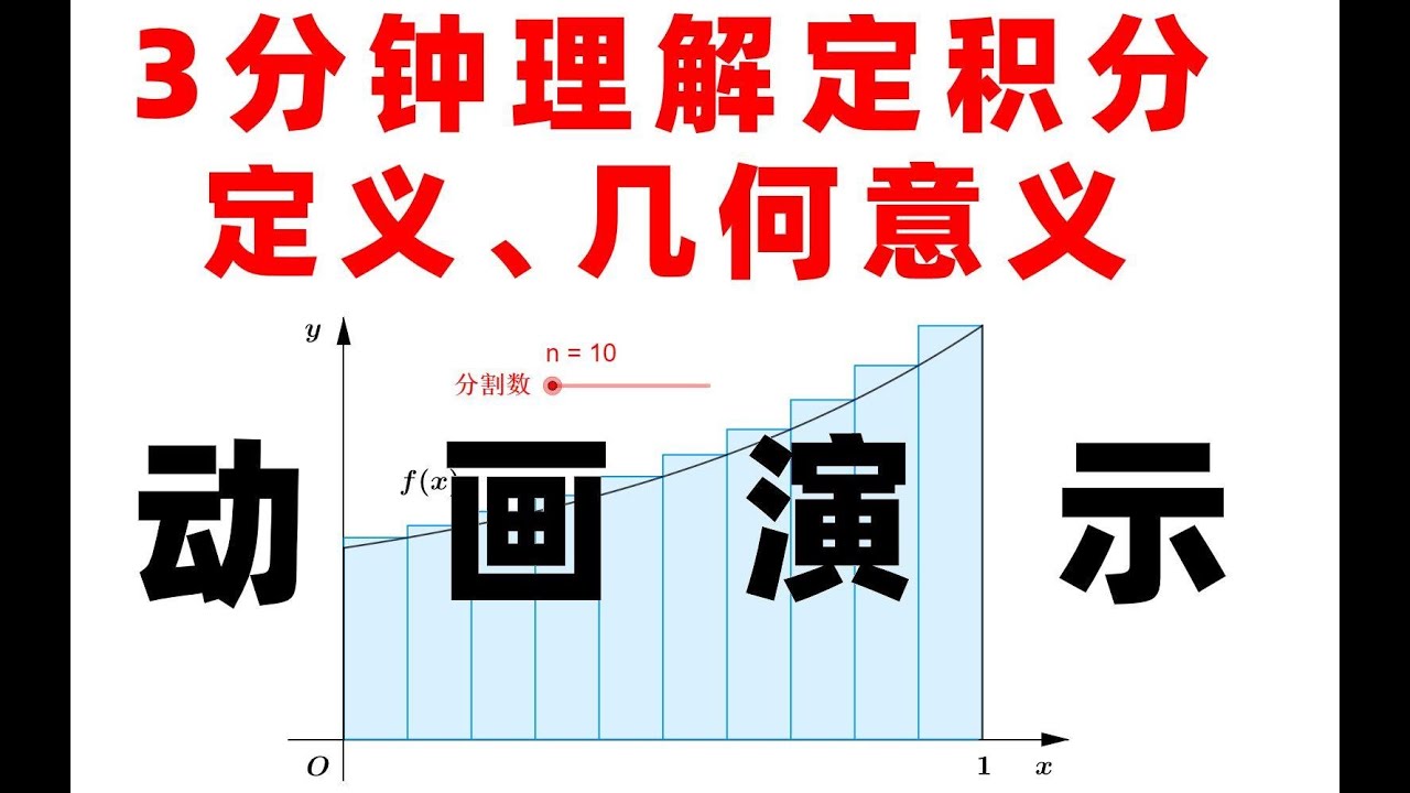 YouTube3:57
Chinese video covering Definite integrals; the current video is in English.
Definite integralsYouTube3:57Visual explanation for Definite integrals, compared with the current whiteboard.
Definite integrals