Riemann sums
The whiteboard connects a curve on [a,b], left-endpoint rectangles and . Adding the rectangle contributions gives a finite approximation to the pictured nonnegative area.
 mathvideo•
Khan Academy connects left-endpoint Riemann sums, finer partitions and the limiting definition of the definite integral, with an explicitly intuitive discussion of dx.
Starting from left-endpoint rectangles, this lesson builds the finite sum with width Δx=(b-a)/n and then adds the limit n→∞ to obtain the definite-integral notation. The same positive curve and interval remain visible as finer rectangles illustrate the limiting idea. The final section relates Δx to dx as an explicitly non-rigorous intuition and discusses other approximation rules. Editorial scope: f is Riemann integrable on the finite interval [a,b], with a<b; continuity is sufficient. Sample points belong to their subintervals and the largest subinterval width tends to zero. For the displayed equal partition, n→∞ ensures this. A nonnegative f gives ordinary area; a sign-changing f gives net signed area. No numerical integral is evaluated.
Generated from the video's visuals and explanation; not verbatim speech.
The whiteboard connects a curve on [a,b], left-endpoint rectangles and . Adding the rectangle contributions gives a finite approximation to the pictured nonnegative area.
Dividing the interval into n equal pieces gives the common width .
The height comes from the left endpoint: . Multiply by to obtain one rectangle contribution.
Left, right and midpoint sums choose one sample value in each subinterval. Unequal widths are also allowed. The lesson additionally mentions the trapezoidal rule; this related quadrature uses the average of endpoint values, rather than the standard single-tag rectangle formula.
The label Riemann Sum points to , identifying this construction as a left-endpoint Riemann sum.
Left, right and midpoint sums choose one sample value in each subinterval. Unequal widths are also allowed. The lesson additionally mentions the trapezoidal rule; this related quadrature uses the average of endpoint values, rather than the standard single-tag rectangle formula.
The portrait is identified as Bernhard Riemann, linking the notation’s name to the mathematician.
The lesson now connects the finite sum to the Riemann integral; the next part develops the limit rather than stopping at the name.
The displayed left-endpoint sum uses and common width . It will be placed inside a limiting process.
Refinement gives convergence under the integrability and shrinking-mesh conditions. This does not guarantee that every increase in the number of rectangles strictly reduces the absolute error.
Editorial scope: f is Riemann integrable on the finite interval [a,b], with a<b; continuity is sufficient. Sample points belong to their subintervals and the largest subinterval width tends to zero. For the displayed equal partition, n→∞ ensures this. A nonnegative f gives ordinary area; a sign-changing f gives net signed area.
The additional sketch uses many narrow rectangles to illustrate in the equal-width construction. This is a visual explanation of convergence, rather than a proof that every finite refinement has smaller error.
The limit is written as . Under the stated integrability conditions this notation names the common limiting value; ordinary area additionally requires nonnegativity.
The explanation begins comparing finite rectangle width with the dx notation; the same video continues this comparison in the following section.
The repeated width markers identify as the finite base width of each equal-partition rectangle.
The author uses an infinitely-small-width picture and explicitly calls it non-rigorous. In the usual real-variable Riemann integral, dx marks the integration variable; it is not a finite rectangle width, a newly defined nonzero infinitesimal real number, or the real number zero. The definition uses limits of finite sums.
Each finite sum multiplies a sampled function value by its subinterval width, then adds the contributions. The integral is the limit of these finite sums; this need not be interpreted as an ordinary series of fixed nonzero infinitesimal real numbers.
Left, right and midpoint sums choose one sample value in each subinterval. Unequal widths are also allowed. The lesson additionally mentions the trapezoidal rule; this related quadrature uses the average of endpoint values, rather than the standard single-tag rectangle formula.
Editorial scope: f is Riemann integrable on the finite interval [a,b], with a<b; continuity is sufficient. Sample points belong to their subintervals and the largest subinterval width tends to zero. For the displayed equal partition, n→∞ ensures this. A nonnegative f gives ordinary area; a sign-changing f gives net signed area. The lesson finishes the definition and leaves techniques for evaluating integrals to subsequent lessons.
The whiteboard connects a curve on [a,b], left-endpoint rectangles and . Adding the rectangle contributions gives a finite approximation to the pictured nonnegative area.
For the specific picture shown, the height of the i-th rectangle is f evaluated at the left endpoint x_{i-1} of that subinterval. That is why the summand contains f(x_{i-1}).
Dividing the interval into n equal pieces gives the common width .
Left, right and midpoint sums choose one sample value in each subinterval. Unequal widths are also allowed. The lesson additionally mentions the trapezoidal rule; this related quadrature uses the average of endpoint values, rather than the standard single-tag rectangle formula.
The portrait and terminology introduce Riemann; the later part of this full video explicitly writes the limit and the integral notation.
The pictured left-endpoint sum is , with equal width on . Other valid tags and shrinking-mesh partitions lead to the same integral when f is Riemann integrable.
Refinement gives convergence under the integrability and shrinking-mesh conditions. This does not guarantee that every increase in the number of rectangles strictly reduces the absolute error.
Editorial scope: f is Riemann integrable on the finite interval [a,b], with a<b; continuity is sufficient. Sample points belong to their subintervals and the largest subinterval width tends to zero. For the displayed equal partition, n→∞ ensures this. A nonnegative f gives ordinary area; a sign-changing f gives net signed area.
Editorial scope: f is Riemann integrable on the finite interval [a,b], with a<b; continuity is sufficient. Sample points belong to their subintervals and the largest subinterval width tends to zero. For the displayed equal partition, n→∞ ensures this. A nonnegative f gives ordinary area; a sign-changing f gives net signed area.
The explanation begins comparing finite rectangle width with the dx notation; the same video continues this comparison in the following section.
In a Riemann sum approximation, the interval is divided into subintervals. The width of each subinterval (and thus the base of each rectangle) is denoted by . For equal subdivisions, .
The author uses an infinitely-small-width picture and explicitly calls it non-rigorous. In the usual real-variable Riemann integral, dx marks the integration variable; it is not a finite rectangle width, a newly defined nonzero infinitesimal real number, or the real number zero. The definition uses limits of finite sums.
Left, right and midpoint sums choose one sample value in each subinterval. Unequal widths are also allowed. The lesson additionally mentions the trapezoidal rule; this related quadrature uses the average of endpoint values, rather than the standard single-tag rectangle formula.
Editorial scope: f is Riemann integrable on the finite interval [a,b], with a<b; continuity is sufficient. Sample points belong to their subintervals and the largest subinterval width tends to zero. For the displayed equal partition, n→∞ ensures this. A nonnegative f gives ordinary area; a sign-changing f gives net signed area.
Explore conditions, steps and evidence. Supplementary explanations are labeled separately from content shown in the video.
The graph is labeled y=f(x) in purple above the plotted curve.
The explanation selects the left endpoint to set the pictured rectangle height.
f(x)
The function whose graph bounds the area being approximated by rectangles.
A real-valued function on an interval [a,b]; the video does not state further regularity assumptions.
The x-axis shows a yellow label a at the left end of the shaded region.
The explanation identifies the interval bounded by a and b.
a
Left endpoint of the interval over which the area is approximated.
A real number serving as the lower boundary of the partition interval.
The x-axis shows a yellow label b at the right end of the shaded region.
The explanation identifies the interval bounded by a and b.
b
Right endpoint of the interval over which the area is approximated.
A real number serving as the upper boundary of the partition interval.
The summation formula has upper index n, and the Δx formula divides by n.
The equal partition gives the common width of the rectangle bases.
n
Number of subintervals or rectangles used in the displayed approximation.
A positive integer; the video does not explicitly state this, but the formulas use it as a counting parameter.
The written formula states “where Δx = (b-a)/n”.
The equal partition gives the common width of the rectangle bases.
Δx
Width of each rectangle in the equal-partition example.
Defined in the displayed formula as (b-a)/n for the shown case.
The summation term is f(x_{i-1}).
The explanation selects the left endpoint to set the pictured rectangle height.
The video does not write a separate formula defining x_{i-1}; its meaning is inferred from the spoken left-endpoint description and the summation notation.
x_{i-1}
Sample point used for the i-th rectangle in the displayed left-endpoint sum; visually corresponds to the left endpoint of that subinterval.
A point in the i-th subinterval of [a,b] under the equal-partition setup.
The sigma notation is written with i=1 below Σ and n above Σ.
i
Summation index running from 1 to n over the rectangles.
Integer index in the displayed sum.
n appears as the upper limit of the summation and in Δx = (b-a)/n.
The lesson uses more and narrower rectangles to illustrate improving approximations.
n
Number of subintervals used in the Riemann sum.
Positive integer; the definition later takes n → ∞.
i appears in the summation index i=1 to n.
i
Summation index labeling one rectangle/subinterval.
x_{i-1} appears inside f(x_{i-1}) in the sum.
The graph shows sample points labeled 1, 2, 3, ..., n under the curve.
No coordinate formula for the partition points is separately written; the displayed and earlier narrated sample is the left endpoint.
x_{i-1}
The left endpoint of the displayed subinterval; the earlier section specifies this sampling choice.
Δx appears multiplied by f(x_{i-1}) in the sum.
The formula states Δx = (b-a)/n.
Δx
Width of each subinterval in the displayed Riemann sum.
a appears as the lower endpoint in Δx = (b-a)/n.
a labels the left endpoint of the interval on the x-axis.
The explanation identifies the interval bounded by a and b.
a
Left endpoint of the integration interval.
The explanation connects the rectangle-area total with the displayed finite summation.
The board shows Σ_{i=1}^{n} f(x_{i-1}) Δx, where Δx = (b-a)/n.
The speaker writes “Riemann Sum” and draws an arrow toward the displayed summation formula.
The clip gives a contextual explanation rather than a fully formal definition of a general Riemann sum.
Left, right and midpoint sums choose one sample value in each subinterval. Unequal widths are also allowed. The lesson additionally mentions the trapezoidal rule; this related quadrature uses the average of endpoint values, rather than the standard single-tag rectangle formula.
The example shown uses an interval [a,b].
The displayed formula uses equal subinterval widths.
The sample points shown correspond to left endpoints.
The explanation selects the left endpoint to set the pictured rectangle height.
The blue rectangles under y=f(x) have heights determined by values on the curve at their left edges.
The summation uses f(x_{i-1}) as the sampled height.
For the specific picture on the board, each rectangle’s height is obtained by evaluating f at the left endpoint of its subinterval. Multiplying those heights by the common width Δx and summing gives the displayed approximation to the area under the curve.
The interval [a,b] is partitioned into n equal subintervals.
Each rectangle uses the left endpoint of its subinterval as the sample point.
The equal partition gives the common width of the rectangle bases.
The board writes Δx = (b-a)/n.
When [a,b] is divided into n equal subintervals, each subinterval has width Δx=(b-a)/n. This is the width used in the displayed rectangle sum.
The partition is uniform.
There are n subintervals between a and b.
The explanation connects the rectangle-area total with the displayed finite summation.
The board shows a summation over rectangle contributions.
The clip reviews the basic strategy of estimating the area under a curve by decomposing the region into rectangles and adding their areas. The displayed sigma notation compactly represents that total.
The region is bounded above by y=f(x) and below by the x-axis on [a,b] in the pictured example.
The lesson discusses other sampling choices and also mentions trapezoidal approximation.
The lesson discusses other sampling choices and also mentions trapezoidal approximation.
The clip names these variants verbally but does not display formulas for right-endpoint, midpoint, trapezoidal, or unequal-partition sums.
Left, right and midpoint sums choose one sample value in each subinterval. Unequal widths are also allowed. The lesson additionally mentions the trapezoidal rule; this related quadrature uses the average of endpoint values, rather than the standard single-tag rectangle formula.
The statement is about the broader class of constructions called Riemann sums.
The displayed formula is only one special case.
Σ_{i=1}^n f(x_{i-1}) Δx, where Δx = (b-a)/n is shown on screen.
Rectangles under y=f(x) on [a,b] are drawn to illustrate the sum.
The explanation connects the rectangle-area total with the displayed finite summation.
The video does not state general conditions on f or on the choice of sample points x_{i-1}.
The clip displays a Riemann sum as the total of rectangle areas f(x_{i-1})Δx for i=1,...,n, with equal subinterval width Δx=(b-a)/n. The speaker emphasizes that this is one example of a Riemann sum, not the only possible one.
Interval endpoints are a and b.
There are n subintervals.
The displayed version uses equal width Δx=(b-a)/n.
lim_{n→∞} Σ_{i=1}^n f(x_{i-1}) Δx is written before the sum.
∫_a^b f(x) dx is written as the resulting notation.
The explanation connects the limit of the finite sums to the definite-integral notation.
The video does not explicitly state existence conditions for the limit or integrability assumptions on f.
Editorial scope: f is Riemann integrable on the finite interval [a,b], with a<b; continuity is sufficient. Sample points belong to their subintervals and the largest subinterval width tends to zero. For the displayed equal partition, n→∞ ensures this. A nonnegative f gives ordinary area; a sign-changing f gives net signed area.
Use a Riemann sum over [a,b].
Take the limit as n→∞.
The result is denoted by the definite integral from a to b.
Editorial scope: f is Riemann integrable on the finite interval [a,b], with a<b; continuity is sufficient. Sample points belong to their subintervals and the largest subinterval width tends to zero. For the displayed equal partition, n→∞ ensures this. A nonnegative f gives ordinary area; a sign-changing f gives net signed area.
The lesson discusses other sampling choices and also mentions trapezoidal approximation.
Left, right and midpoint sums choose one sample value in each subinterval. Unequal widths are also allowed. The lesson additionally mentions the trapezoidal rule; this related quadrature uses the average of endpoint values, rather than the standard single-tag rectangle formula.
Applies when approximating definite integrals using finite sums.
The explanation connects the limit of the finite sums to the definite-integral notation.
The equation is displayed.
Editorial scope: f is Riemann integrable on the finite interval [a,b], with a<b; continuity is sufficient. Sample points belong to their subintervals and the largest subinterval width tends to zero. For the displayed equal partition, n→∞ ensures this. A nonnegative f gives ordinary area; a sign-changing f gives net signed area.
The limit must exist.
n represents the number of subintervals.
represents the width of the subintervals.
Editorial scope: f is Riemann integrable on the finite interval [a,b], with a<b; continuity is sufficient. Sample points belong to their subintervals and the largest subinterval width tends to zero. For the displayed equal partition, n→∞ ensures this. A nonnegative f gives ordinary area; a sign-changing f gives net signed area.
The explanation connects the limit of the finite sums to the definite-integral notation.
At this early item’s time the next part has not yet been developed; it is continued later in the same complete video.
The speaker states that the Riemann sum is used to define the Riemann integral.
The context is a first-year calculus course.
The discussion concerns the standard role of Riemann sums in integration theory.
No explicit quantifier is stated in the clip.
The portrait is identified as Riemann, linking his name to the terminology.
A portrait is shown with the handwritten label “Bernhard Riemann”.
The clip attributes the name “Riemann sums” to Bernhard Riemann.
Universal naming attribution as stated by the speaker; no formal logical quantifier is given.
The lecturer introduces the Riemann approach as a formal definition used in calculus.
This is presented as the lecturer's characterization rather than a proved statement within the clip.
The Riemann integral is presented as a mainstream formal or rigorous definition of the integral.
No explicit quantifier is stated in the clip.
The lesson uses more and narrower rectangles to illustrate improving approximations.
The initial drawing shows finitely many rectangles approximating the area under the curve.
The clip does not prove this monotonic improvement claim; it is stated verbally.
Refinement gives convergence under the integrability and shrinking-mesh conditions. This does not guarantee that every increase in the number of rectangles strictly reduces the absolute error.
A Riemann sum is being used to approximate the area under a curve on [a,b].
Editorial scope: f is Riemann integrable on the finite interval [a,b], with a<b; continuity is sufficient. Sample points belong to their subintervals and the largest subinterval width tends to zero. For the displayed equal partition, n→∞ ensures this. A nonnegative f gives ordinary area; a sign-changing f gives net signed area.
For Riemann-integrable f and tagged partitions whose mesh tends to zero; no stepwise strict-error comparison asserted.
The explanation says the limiting idea is not restricted to the one drawn sampling choice.
The clip does not specify the precise class of allowed Riemann sums or prove independence of the choice.
Editorial scope: f is Riemann integrable on the finite interval [a,b], with a<b; continuity is sufficient. Sample points belong to their subintervals and the largest subinterval width tends to zero. For the displayed equal partition, n→∞ ensures this. A nonnegative f gives ordinary area; a sign-changing f gives net signed area.
Editorial scope: f is Riemann integrable on the finite interval [a,b], with a<b; continuity is sufficient. Sample points belong to their subintervals and the largest subinterval width tends to zero. For the displayed equal partition, n→∞ ensures this. A nonnegative f gives ordinary area; a sign-changing f gives net signed area.
All valid tags and shrinking-mesh partitions for a Riemann-integrable function.
The explanation connects the rectangle-area total with the displayed finite summation.
The board displays Σ_{i=1}^{n} f(x_{i-1}) Δx with Δx=(b-a)/n.
The rectangles under y=f(x) visually match a left-endpoint construction.
The clip does not write out the intermediate algebraic derivation step by step; it presents the final sigma form directly.
Start with the geometric picture of several rectangles approximating the area under y=f(x) on [a,b].
Uses the rectangle-width and sampling construction explained in the lesson.
Because the interval is equally partitioned into n pieces, each rectangle has the same width.
Explicitly stated in the audio and written on the board.
For the i-th rectangle, the height is taken from the function value at the left endpoint of that subinterval.
Explicitly stated in the audio and consistent with the diagram.
Adding the areas of all n rectangles gives the displayed finite sum.
Area of each rectangle is height times width; summing over i yields the sigma expression.
The pictured left-endpoint equal-width rectangle approximation is summarized by the formula Σ_{i=1}^{n} f(x_{i-1})Δx with Δx=(b-a)/n.
lim_{n→∞} is added in front of the Riemann sum.
A second diagram is drawn with many more narrow rectangles under the curve.
The explanation connects the limit of the finite sums to the definite-integral notation.
The final notation ∫_a^b f(x) dx is written.
The derivation is conceptual and visual; the clip does not provide an epsilon-delta proof or discuss convergence criteria.
Start with a finite Riemann sum representing the total area of n rectangles under the curve.
This is the formula already written on screen and identified verbally as a Riemann sum.
For the equal partition, increasing n makes all subinterval widths tend to zero; with Riemann integrability the sums converge.
Uses the rectangle-width and sampling construction explained in the lesson.
Denote the common limit by the definite integral; the positive example permits an ordinary-area interpretation.
Uses the rectangle-width and sampling construction explained in the lesson.
Editorial scope: f is Riemann integrable on the finite interval [a,b], with a<b; continuity is sufficient. Sample points belong to their subintervals and the largest subinterval width tends to zero. For the displayed equal partition, n→∞ ensures this. A nonnegative f gives ordinary area; a sign-changing f gives net signed area.
The explanation links shrinking finite widths to the dx notation and later cautions that its infinitesimal picture is intuition.
Visual annotation 'infinitely small' added to dx.
Speaker notes this is not a rigorous way of thinking about it.
Start with the finite width of a rectangle in a Riemann sum.
Definition of Riemann sum components.
Consider the width becoming infinitely small.
Uses the rectangle-width and sampling construction explained in the lesson.
The author uses an infinitely-small-width picture and explicitly calls it non-rigorous. In the usual real-variable Riemann integral, dx marks the integration variable; it is not a finite rectangle width, a newly defined nonzero infinitesimal real number, or the real number zero. The definition uses limits of finite sums.
Notation for the differential.
The author uses an infinitely-small-width picture and explicitly calls it non-rigorous. In the usual real-variable Riemann integral, dx marks the integration variable; it is not a finite rectangle width, a newly defined nonzero infinitesimal real number, or the real number zero. The definition uses limits of finite sums.
A graph of y=f(x) over [a,b] is shown with several blue rectangles beneath the curve.
The board writes Σ_{i=1}^{n} f(x_{i-1}) Δx, where Δx = (b-a)/n.
The explanation connects the rectangle-area total with the displayed finite summation.
No numerical function, interval endpoints, or value of n are specified, so no numeric answer can be computed from the clip.
Approximate the area under y=f(x) from x=a to x=b using equally spaced rectangles whose heights come from left endpoints.
Function graph y=f(x).
Interval endpoints a and b.
n equal subintervals.
Rectangle heights use left endpoints x_{i-1}.
Express the rectangle-area approximation in sigma notation and identify it as a Riemann sum.
Partition [a,b] into n equal subintervals, giving each rectangle the same width.
Uses the rectangle-width and sampling construction explained in the lesson.
Use the function value at the left endpoint of the i-th subinterval as the rectangle height.
Uses the rectangle-width and sampling construction explained in the lesson.
Sum the areas of all rectangles to obtain the approximation.
Follows from adding height times width over all subintervals.
Label the resulting finite sum as a Riemann sum.
Uses the rectangle-width and sampling construction explained in the lesson.
The displayed approximation is the Riemann sum with .
The formula matches the visual construction: equal-width rectangles under y=f(x) on [a,b] with heights taken at left endpoints.
The screen shows a portrait labeled “Bernhard Riemann” on the left, a coordinate graph with y=f(x) and rectangles on the upper right, and a summation formula below.
A cursor moves among the portrait, the rectangles, the labels a and b, and the formula.
Portrait labeled “Bernhard Riemann”.
Coordinate axes x and y.
Curve labeled y=f(x).
Blue rectangles under the curve on [a,b].
Formula Σ_{i=1}^{n} f(x_{i-1}) Δx, where Δx=(b-a)/n.
The cursor points first to the rectangles and interval endpoints.
It then moves to the summation formula.
Later it points to the portrait and the handwritten label “Riemann Sum”.
The graph remains on [a,b] throughout.
The displayed formula remains the same throughout the clip.
The rectangles continue to represent a left-endpoint equal-width construction.
The visual arrangement links the historical figure, the geometric rectangle picture, and the symbolic Riemann-sum formula as three representations of the same idea.
Handwritten text appears near the formula.
The new label reads “Riemann Sum” with an arrow pointing toward the summation expression.
Exact stroke-by-stroke timing of the handwriting is approximate from the sampled frames.
Handwritten words “Riemann Sum”.
Arrow pointing to the summation formula.
The phrase “Riemann Sum” is written on the board.
An arrow is drawn from the phrase to the formula.
The underlying formula Σ_{i=1}^{n} f(x_{i-1}) Δx does not change.
This annotation explicitly identifies the displayed finite sum as an instance of a Riemann sum.
A portrait labeled 'Bernhard Riemann' appears at left; a graph of y=f(x) with rectangles on [a,b] appears center; the formula Σ_{i=1}^n f(x_{i-1})Δx, where Δx=(b-a)/n, is written below; 'Riemann Sum' is written at right with an arrow.
Portrait labeled Bernhard Riemann
Coordinate axes x and y
Curve labeled y=f(x)
Rectangles under the curve on [a,b]
Formula Σ_{i=1}^n f(x_{i-1})Δx
Definition Δx=(b-a)/n
Label 'Riemann Sum'
The cursor points among the summation symbol, the rectangles, and the formula components.
The interval endpoints a and b remain fixed.
The curve y=f(x) remains the same in the first diagram.
The board visually links the geometric rectangle approximation to the algebraic Riemann-sum formula.
A new coordinate system is drawn at lower left, then a curve and many narrow blue rectangles between a and b.
The lesson uses more and narrower rectangles to illustrate improving approximations.
The exact number of rectangles is not specified; the drawing is schematic.
New x-y axes
Curve on [a,b]
Many narrow blue rectangles
Labels a and b
A second diagram is added below the original content.
The rectangles are much thinner and more numerous than in the first diagram.
The conceptual interval remains from a to b.
The purpose remains approximating area under the curve.
Editorial scope: f is Riemann integrable on the finite interval [a,b], with a<b; continuity is sufficient. Sample points belong to their subintervals and the largest subinterval width tends to zero. For the displayed equal partition, n→∞ ensures this. A nonnegative f gives ordinary area; a sign-changing f gives net signed area.
∫_a^b f(x) dx is written to the right of the limit expression.
The explanation connects the limit of the finite sums to the definite-integral notation.
Expression lim_{n→∞} Σ_{i=1}^n f(x_{i-1})Δx
New notation ∫_a^b f(x) dx
The integral notation is added after the limit expression is established.
The same interval [a,b] and function f are referenced.
Editorial scope: f is Riemann integrable on the finite interval [a,b], with a<b; continuity is sufficient. Sample points belong to their subintervals and the largest subinterval width tends to zero. For the displayed equal partition, n→∞ ensures this. A nonnegative f gives ordinary area; a sign-changing f gives net signed area.
The words 'infinitely small' are handwritten next to the dx term in the integral formula.
Text 'infinitely small'
Formula term dx
Text appears on screen.
The rest of the formula remains unchanged.
The author uses an infinitely-small-width picture and explicitly calls it non-rigorous. In the usual real-variable Riemann integral, dx marks the integration variable; it is not a finite rectangle width, a newly defined nonzero infinitesimal real number, or the real number zero. The definition uses limits of finite sums.
The lesson discusses other sampling choices and also mentions trapezoidal approximation.
The lesson discusses other sampling choices and also mentions trapezoidal approximation.
One might think a Riemann sum must always use equal-width rectangles with left-endpoint heights.
The clip states that the displayed construction is only one particular instance; more general Riemann sums allow different sample points and unequal partitions.
The explanation says the limiting idea is not restricted to the one drawn sampling choice.
One might think the specific sum Σ_{i=1}^n f(x_{i-1})Δx with Δx=(b-a)/n is the only Riemann sum that matters.
Editorial scope: f is Riemann integrable on the finite interval [a,b], with a<b; continuity is sufficient. Sample points belong to their subintervals and the largest subinterval width tends to zero. For the displayed equal partition, n→∞ ensures this. A nonnegative f gives ordinary area; a sign-changing f gives net signed area.
The lesson contrasts a finite rectangle approximation with the limit represented by the integral.
Increasing n is shown to improve the approximation.
This misconception is inferred from the contrast made in the video rather than named directly.
A finite sum must always equal the integral, or conversely can never equal it.
Finite sums are approximations in general; special functions and sampling choices can give equality already. The limiting definition ensures the common integral under the integrability and shrinking-mesh conditions.
The explanation links shrinking finite widths to the dx notation and later cautions that its infinitesimal picture is intuition.
Thinking of dx simply as an 'infinitely small number' is mathematically rigorous.
The author uses an infinitely-small-width picture and explicitly calls it non-rigorous. In the usual real-variable Riemann integral, dx marks the integration variable; it is not a finite rectangle width, a newly defined nonzero infinitesimal real number, or the real number zero. The definition uses limits of finite sums.
The explanation connects the rectangle-area total with the displayed finite summation.
The board shows the sigma expression corresponding to the rectangle picture.
The general method of summing rectangle areas is applied here through the specific left-endpoint rule shown on the board.
The lesson discusses other sampling choices and also mentions trapezoidal approximation.
The label “Riemann Sum” is attached to the specific formula.
The named concept “Riemann sum” generalizes the specific left-endpoint equal-width formula shown in the example.
The explanation connects the limit of the finite sums to the definite-integral notation.
At this early item’s time the next part has not yet been developed; it is continued later in the same complete video.
The first section announces the integral connection; the subsequent sections write the limit and continue the dx discussion.
lim_{n→∞} Σ_{i=1}^n f(x_{i-1})Δx = ∫_a^b f(x) dx is assembled across the board.
The explanation connects the limit of the finite sums to the definite-integral notation.
Editorial scope: f is Riemann integrable on the finite interval [a,b], with a<b; continuity is sufficient. Sample points belong to their subintervals and the largest subinterval width tends to zero. For the displayed equal partition, n→∞ ensures this. A nonnegative f gives ordinary area; a sign-changing f gives net signed area.
The explanation links shrinking finite widths to the dx notation and later cautions that its infinitesimal picture is intuition.
Δx appears in the sum and dx appears in the integral notation.
At this early item’s time the next part has not yet been developed; it is continued later in the same complete video.
The width-to-notation comparison begins here and continues later in the complete video.
The explanation links shrinking finite widths to the dx notation and later cautions that its infinitesimal picture is intuition.
The author uses an infinitely-small-width picture and explicitly calls it non-rigorous. In the usual real-variable Riemann integral, dx marks the integration variable; it is not a finite rectangle width, a newly defined nonzero infinitesimal real number, or the real number zero. The definition uses limits of finite sums.
The explanation connects the limit of the finite sums to the definite-integral notation.
Editorial scope: f is Riemann integrable on the finite interval [a,b], with a<b; continuity is sufficient. Sample points belong to their subintervals and the largest subinterval width tends to zero. For the displayed equal partition, n→∞ ensures this. A nonnegative f gives ordinary area; a sign-changing f gives net signed area.
The explanation connects the rectangle-area total with the displayed finite summation.
The board writes “Riemann Sum” next to the formula.
The explanation selects the left endpoint to set the pictured rectangle height.
The summation uses f(x_{i-1}).
The equal partition gives the common width of the rectangle bases.
The board writes Δx=(b-a)/n.
The lesson discusses other sampling choices and also mentions trapezoidal approximation.
The explanation connects the limit of the finite sums to the definite-integral notation.
At this early item’s time the next part has not yet been developed; it is continued later in the same complete video.
Σ_{i=1}^n f(x_{i-1})Δx, where Δx=(b-a)/n is shown.
The explanation connects the rectangle-area total with the displayed finite summation.
lim_{n→∞} Σ_{i=1}^n f(x_{i-1})Δx = ∫_a^b f(x) dx is written.
The explanation connects the limit of the finite sums to the definite-integral notation.
The lesson uses more and narrower rectangles to illustrate improving approximations.
A second diagram shows many more narrow rectangles.
The explanation says the limiting idea is not restricted to the one drawn sampling choice.
The explanation links shrinking finite widths to the dx notation and later cautions that its infinitesimal picture is intuition.
The explanation connects the limit of the finite sums to the definite-integral notation.
Covered · Audio introduces the review of approximating area under a curve by summing rectangle areas; the graph and formula are already visible.
Covered · Speaker explains equal widths and the partition of [a,b]; the formula Δx=(b-a)/n is visible.
Covered · Speaker identifies the heights as left-endpoint function values, matching f(x_{i-1}) in the displayed sum.
Covered · Speaker mentions other variants such as right endpoints, midpoints, and trapezoids as related constructions.
Covered · Speaker names the displayed construction as a Riemann sum and writes the label with an arrow to the formula.
Covered · Speaker stresses that Riemann sums are more general and need not use equal spacing.
Covered · Speaker identifies Bernhard Riemann from the portrait and states that Riemann sums are used to define the Riemann integral.
Covered · Opening explanation of the displayed Riemann sum, its formula, and the claim that larger n improves the approximation.
Covered · The clip adds the limit as n→∞, draws a finer-rectangle diagram, introduces ∫_a^b f(x) dx, and begins to relate Δx to dx before ending.
Covered · Identification of delta x as rectangle width.
Covered · Conceptual explanation of dx and its relation to delta x.
Covered · Summary of the summation process (function times delta x summed from a to b).
Covered · Discussion of different Riemann sum types and the formal definition of the integral as a limit.
Editorial scope: f is Riemann integrable on the finite interval [a,b], with a<b; continuity is sufficient. Sample points belong to their subintervals and the largest subinterval width tends to zero. For the displayed equal partition, n→∞ ensures this. A nonnegative f gives ordinary area; a sign-changing f gives net signed area.
 YouTube2:28
Another explanation of Definite integrals.
Definite integrals YouTube4:16
Another explanation of Definite integrals.
Definite integrals YouTube3:30
Another explanation of Definite integrals.
Definite integrals Bilibili7:03
Next in Calculus: Definite integrals → Improper integrals.
Improper integrals · View learning sequence YouTube2:26
Prerequisite in Calculus: Limits → Definite integrals.
Limits · View learning sequence YouTube2:38
Prerequisite in Calculus: Limits → Definite integrals.
Limits · View learning sequence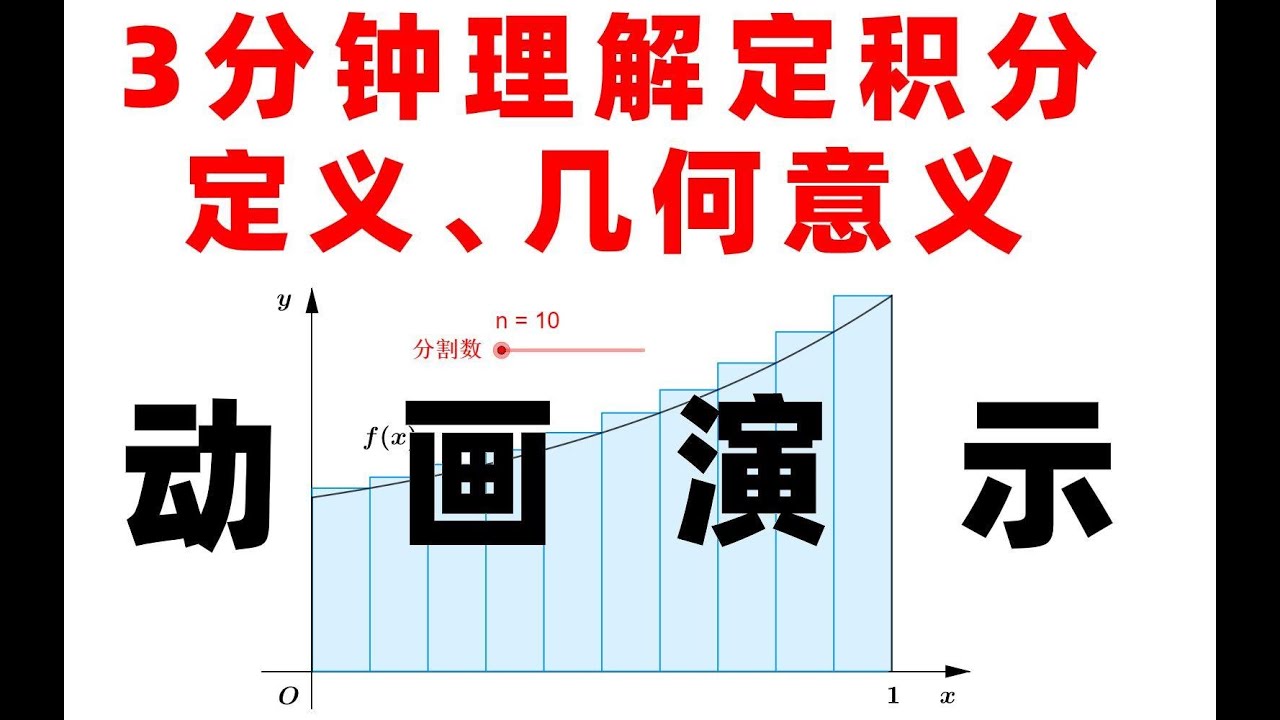 YouTube3:57
Chinese video covering Definite integrals; the current video is in English.
Definite integralsYouTube3:57Visual explanation for Definite integrals, compared with the current whiteboard.
Definite integrals