Fourier Series
A mathematical concept that allows any function to be written as a sum of sine and cosine waves.
Up and Atom · YouTube · 14:47
This video introduces the concepts of Fourier series and Fourier transforms, explaining how suitable periodic functions can be expanded as a sum of sine and cosine waves. It visually demonstrates the process of adding functions together and shows how infinite sums of waves can approximate complex shapes like square and sawtooth waves. This 180-second clip gives an introductory, visual explanation of Fourier methods through applications. It first compares a square wave and a sawtooth wave using three-term sine expansions, showing that the differing coefficient of the term can identify which waveform is which. It then extends the idea to outline analysis for image analysis and shape recognition, using an apple and a pizza slice as examples. Next, it explains that a signal can be viewed either as amplitude versus time or as a sum of frequencies, and demonstrates audio filtering by removing unwanted high-pitched components and recombining the rest. Finally, it introduces the Fourier transform as a tool that maps an amplitude-versus-time function to an amplitude-versus-frequency representation by decomposing the function into sine and cosine waves and retaining only amplitude-frequency pairings. This 180-second excerpt explains the Fourier transform by moving from a bar-chart picture of frequency components to the explicit formula . It first shows that a square wave's early Fourier-series terms correspond to bars of heights 1, 0, and at frequencies 1, 2, and 3. The presenter then uses Euler's formula to show where sine and cosine enter the transform. In the worked example at frequency 3, the clip argues that because the square wave starts in phase with sine waves at , the cosine term can be dropped for that example, leaving the integral of . The final visuals interpret this product as a pointwise correlation test, illustrated by overlaying the square wave and sine wave and zooming to where both have value 1. This 180-second clip explains Fourier analysis through a square-wave example. It first multiplies the square wave by point by point, then integrates those products to judge overall correlation. A positive result means the harmonic is present; after normalization the video gives the coefficient . It then explains visually why only odd sine harmonics survive, why even harmonics and cosine terms cancel, and finally recasts the whole procedure as changing from a time description to a frequency description using an orthogonal sine-cosine basis. This introductory segment defines algorithms as step-by-step instructions for managing complex processes, highlighting their necessity in applying Fourier transforms to real-world data like video playback. It illustrates the widespread, often invisible, use of algorithms in modern technology through examples ranging from audio engineering to medical imaging, before transitioning into a promotional message for educational streaming platforms. Editorial correction: the video labels the sine correlation integral as , but the complete complex Fourier coefficient also includes the factor -i and a normalization convention. For an odd square wave of amplitude ±1 on [-π,π], and ; the displayed is the ratio , not the unnormalized integral.
Use the learning inspector for key ideas and moments, or open the reading tabs for the complete notes.
Generated from the video's visuals and explanation; not verbatim speech.
The video begins with a sponsor message for Curiosity Stream and Nebula.
The host, Jade, introduces the topic of Fourier series and Fourier transforms, stating that any function can be written as a sum of sine and cosine waves.
Jade addresses potential skepticism about representing sharp-cornered functions like square waves using smooth sine and cosine waves.
The video explains the basic concept of adding two functions together by summing their y-values at each x-value, using and as examples.
Specific calculations are shown for adding and at and .
The resulting graph of the added functions is shown, and Jade explains how the sum behaves when the original functions are positive or negative.
The video demonstrates how adding more terms with smaller amplitudes progressively approximates a square wave, introducing the concept of infinite sums in Fourier series.
Another example is provided, showing how a Fourier series can approximate a sawtooth wave using the first few terms: .
Jade concludes by addressing the practical utility of Fourier series, noting that in many real-world applications, an approximate solution is sufficient.
The clip opens with a practical question: suppose a program is given two periodic functions and needs to tell them apart. On screen, the two example functions are a square wave and a sawtooth wave.
To answer that question, the video writes the first few Fourier-series terms for each waveform. For the square wave it displays , and for the sawtooth wave it displays .
The key observation is immediate: the first and third displayed coefficients match, but the second coefficient differs. Therefore, in this example, the amplitude of the term alone is enough for a program to identify which waveform is which.
The narrator then adds a caution: for such a simple pair of waves, computing a full Fourier series may be more effort than necessary. Still, the same decomposition idea is useful more broadly.
That broader use is pattern and shape recognition. The screen replaces the graphs with an apple and a pizza slice, and the explanation says their outlines can be analyzed with the same technique to decide which object is which.
From there the clip names the application directly: Fourier analysis is an important tool in image analysis and shape recognition.
The next conceptual obstacle is identified: the difficult part is not the idea of decomposition itself, but figuring out how to find the Fourier series, meaning which waves combine to produce the desired shape.
The video illustrates this difficulty with a question mark over multiple waveforms, emphasizing that constructing a shape from waves is nontrivial, whether the target is a pizza outline or a square wave.
Before addressing that harder problem, the clip pivots to one more useful feature of the Fourier series: the distinction between a function over time and its representation as a sum of frequencies.
A square wave is shown on a TIME axis, while below it a stack of colored sinusoids is labeled as a sum of many frequencies. This visual contrast sets up the next application.
The example becomes audio filtering. Imagine a recording contaminated by a high-pitched sound. If the recording is decomposed into frequency components, the unwanted high-pitched terms can be removed and the remaining terms recombined.
The animation makes that process concrete: a composite waveform splits into several component waves, some components disappear, and the rest are added back to reconstruct a cleaner signal.
This leads to the Fourier transform, introduced as a tool associated with the Fourier series. The clip says it can identify which frequencies, or which sines and cosines, are present in a function.
More importantly, the transform can also remove selected frequencies without first requiring the full Fourier series to be written out. That is the mathematical justification for the filtering example just shown.
The final explanation states the basic input-output idea of the Fourier transform: you provide an amplitude-versus-time function, and the transform returns the same information as an amplitude-versus-frequency function.
Why does that work? Because the transform decomposes the function into sine and cosine waves. However, instead of displaying every wave separately, the useful summary is the pairing of each frequency with its amplitude.
The closing animation condenses a messy stack of sinusoids into vertical spikes on a FREQUENCY axis. The takeaway is that the frequency-domain plot is a compact rewrite of the decomposition, keeping only the amplitudes and frequencies that matter.
The clip opens on a white chart whose vertical axis is labeled AMPLITUDE and horizontal axis FREQUENCY. Several blue vertical bars stand at different horizontal positions. The narration explains that each wave has been collapsed into one bar: height records amplitude, and position records frequency. This establishes the basic visual language for the rest of the segment.
The camera pulls back to a red tool labeled FOURIER TRANSFORM, flanked by two cards. The left card, labeled TIME, shows a square wave; the right card, labeled FREQUENCY, shows the bar chart. The speaker summarizes the key idea: the Fourier transform output is a frequency-domain view of the original time-domain function. The metaphor is that the same signal can be described either as a waveform over time or as a set of component strengths over frequency.
A presenter appears beside a monitor titled 'Fourier Series of a Square Wave'. On the screen, the formula builds to , while yellow arrows connect these terms to bars at frequencies 1, 2, and 3. The reasoning is direct: coefficient 1 gives a tall bar at frequency 1, coefficient 0 gives no bar at frequency 2, and coefficient gives a shorter bar at frequency 3. This turns the algebraic series into a spectral picture.
The scene changes to the formula . White highlights isolate the parts in turn. The speaker identifies as the Fourier transform, the quantity being solved for, and as the original time function. A square-wave inset appears under , tying the abstract symbol to the example waveform. The remaining factors, the exponential and the integral, are introduced as the mechanism that extracts frequency information.
To explain why sine and cosine appear, the video displays Euler's formula , alongside a circular-motion graphic projecting sinusoidal traces. The next line substitutes this identity into the transform, yielding . The mathematical point is that the complex exponential kernel is exactly a packaged pair of trigonometric functions, so the transform integral naturally tests the signal against cosine and sine components.
The lesson then specializes to frequency 3 with the header . A green sine wave of frequency 3 is drawn above an orange square wave. The narration explains why the imaginary part matters in general: different phases can require both components. But for this square wave, the speaker states that it starts in phase with sine waves at , so the cosine term is dropped for the example and the formula is rewritten as . Editorial correction: the video labels the sine correlation integral as , but the complete complex Fourier coefficient also includes the factor -i and a normalization convention. For an odd square wave of amplitude ±1 on [-π,π], and ; the displayed is the ratio , not the unnormalized integral.
With the simplified integrand on screen, the speaker interprets procedurally: at each x, multiply the square-wave height by the sine-wave height at the same x. The accumulated result is described as a measure of correlation between the two waves. The visuals reinforce this by overlaying the curves and then zooming to , where the square wave is labeled at height 1 and the sine wave is at its peak. Thus the local product is , illustrating how matching shapes contribute positively to the integral. The clip stops before completing the full evaluation of .
The clip opens on a graph with an orange square wave and a green sine wave plotted together. Dotted vertical markers pick out sample -values, and the video multiplies the two function values at those points. The visible examples are , , , , and . The spoken rule is simple: positive product means local agreement, negative product means local opposition, and zero means no local contribution.
The presenter then shifts from isolated samples to the whole interval. The formula is treated as the continuous version of adding all those pointwise products. Blue and red shaded regions accumulate under the curve while a vertical meter tracks the running total. This visual makes the next rule natural: if the final total is positive, the test wave is overall correlated with the square wave; if it is zero, there is no net contribution; if it is negative, the contribution enters with the opposite sign. Editorial correction: the video labels the sine correlation integral as , but the complete complex Fourier coefficient also includes the factor -i and a normalization convention. For an odd square wave of amplitude ±1 on [-π,π], and ; the displayed is the ratio , not the unnormalized integral.
For this particular square-wave example, the accumulated total is positive, so the third harmonic is present. The video then states the normalized coefficient: only one third of the amplitude of is used. On screen this appears as and as the circled term inside the displayed series. The normalization computation itself is not derived here; the clip gives the result and connects it to the series expression. Editorial correction: the video labels the sine correlation integral as , but the complete complex Fourier coefficient also includes the factor -i and a normalization convention. For an odd square wave of amplitude ±1 on [-π,π], and ; the displayed is the ratio , not the unnormalized integral.
Next the explanation broadens from one harmonic to the whole pattern. A displayed series, , shows only odd sine terms. The accompanying panels labeled ODD FREQUENCIES, EVEN FREQUENCIES, and COSINE WAVES explain why. For odd frequencies, the positive and negative correlation humps do not balance, so the integral stays positive. For even frequencies, the humps cancel exactly, giving zero. The same cancellation idea is then used to explain why cosine terms do not appear in this square-wave series.
Having explained the Fourier-series case, the speaker generalizes to the Fourier transform: the same correlation procedure can be applied at any frequency to reveal which frequencies are present in a function. The visual language changes from flat graphs to a rotating 3D-style scene and then to a Swiss-army-knife graphic labeled FOURIER TRANSFORM. One card shows AMPLITUDE versus TIME, and another shows AMPLITUDE versus FREQUENCY, summarizing the move from a time description to a frequency description.
The final conceptual reframing is that Fourier analysis is like changing basis in an infinite-dimensional function space. Just as one can describe the same vector using different coordinates, one can describe the same function either by its amplitudes across time positions or by its amplitudes across frequency values. The clip closes by saying this works because sine and cosine waves form an orthogonal basis, so they can be combined to represent functions in the same spirit that orthogonal vectors span a vector space.
The segment begins by contextualizing the previous discussion on vector spaces. While transforming functions between bases is mathematically powerful, the speaker notes a practical limitation: pure algebraic methods require a known mathematical formula for the input function.
In real-world scenarios, such as playing a video file, we rarely have a perfect mathematical description. Instead, we deal with 'raw data' which is messy and complex. Computers rely on Fourier transforms to process this data for playback.
To bridge the gap between ideal math and messy reality, we need algorithms. The speaker provides a clear definition: algorithms are step-by-step instructions that decompose a complicated process into small, manageable tasks.
This concept is linked back to earlier examples. Both pattern recognition and audio engineering require algorithms to function effectively on real data. The speaker emphasizes that algorithms operate quietly behind the scenes in many aspects of daily life.
The remainder of the clip serves as a promotional interlude. A montage of clips from a documentary illustrates diverse algorithmic applications, including recommendation systems, dating matches, medical transplants, and logistics. The speaker then details a sponsorship offer for CuriosityStream and Nebula, concluding the video with thanks to supporters.
A mathematical concept that allows any function to be written as a sum of sine and cosine waves.
An accompanying mathematical idea to the Fourier series, used in various applications like digital music and image recognition.
To add two functions, you take the y-values of each function at a specific x-value and add them together to get the new y-value for the resulting function.
By adding infinitely many waves, you can reach an exact solution for a square wave using a Fourier series.
The Fourier series can also approximate a sawtooth wave.
The clip introduces Fourier series through a concrete comparison task. A square wave and a sawtooth wave are each represented by the first few sine terms shown on screen. The square-wave example is , while the sawtooth-wave example is . Since the first and third displayed coefficients agree but the second differs, the amplitude of the term is enough to distinguish the two shown cases.
After the simple waveform example, the video generalizes the same idea to outlines of objects. An apple and a pizza slice are used as visual examples to show that Fourier analysis can help compare shapes by analyzing their boundary structure. The clip does not derive an outline algorithm here; it presents the application conceptually as image analysis and shape recognition.
The narration identifies the main practical difficulty: once you accept that a shape can be decomposed into waves, the remaining challenge is determining which waves combine to produce the desired form. The question-mark animation over multiple sinusoids visually represents this inverse problem of choosing the correct frequency content for a target shape.
The clip contrasts two ways of describing the same signal. One view is amplitude as a function of time, shown by the square-wave graph on a TIME axis. The other view is the signal as a sum of many frequencies, shown by several colored sinusoids stacked below. This prepares the transition from Fourier-series intuition to transform-based frequency analysis.
Using an audio example, the video explains that if a recording contains an unwanted high-pitched sound, one can decompose the signal into frequency components, remove the terms associated with that pitch, and recombine the remaining terms. The result is the original recording without the distracting high-frequency component. This is presented as a direct practical use of Fourier-style decomposition.
The Fourier transform is introduced as a tool associated with the Fourier series. Its role in this clip is to identify which frequencies, or which sine and cosine components, are present in a function. The video also stresses that the transform can remove selected frequencies even without first explicitly constructing the full Fourier series.
The final conceptual card explains the transform as a mapping between representations. The input is an amplitude-versus-time function; the output is the same information expressed as amplitude versus frequency. The visual metaphor is a machine that accepts a time-domain graph and produces a spike spectrum, summarizing the decomposition by frequency and amplitude alone.
Type: definition. Each sinusoidal component is replaced by one vertical bar. Bar height encodes amplitude and bar position encodes frequency. This is the visual convention used throughout the clip to translate a sum of waves into a spectrum-like picture. Evidence: 00:00-00:13. Related to the later square-wave example at 00:23-00:57.
Type: definition. The video states that the transform output is not a new unrelated object but a representation of the same time-domain function in frequency coordinates. The Swiss-army-knife graphic contrasts a TIME card with a FREQUENCY card. Evidence: 00:14-00:22.
Type: formula. The screen shows the truncated series for the square wave and the narration names the expected terms. The coefficient pattern is then mapped onto bars at frequencies 1, 2, and 3. Evidence: 00:23-00:57. Prerequisite: understanding the bar-chart encoding from 00:00-00:13.
Type: formula. The presenter displays the transform as an integral of the time function against a complex exponential. The narration identifies as the desired output and as the original time function. The clip does not state integration limits or normalization conventions. Evidence: 00:58-00:98.
Type: formula. The exponential factor in the transform is rewritten using Euler's identity, making clear that one complex exponential contains a cosine part and a sine part. A circular-motion graphic accompanies the algebra. Evidence: 00:99-00:112.
Type: formula. After applying Euler's formula, the transform is rewritten so the integrand explicitly contains []. This is the intermediate form used before the frequency-3 example. Evidence: 00:113-00:129. Depends on the previous two cards.
Type: method. The narration says the imaginary component is needed in general to handle phase differences, but this square wave starts in phase with sine waves at . Therefore, for this example only, the cosine contribution is discarded and the sine contribution is treated as the real component of interest. Evidence: 00:130-00:163. This simplification is example-specific, not a universal rule. The screen writes for a sine-only integral. This is pedagogical shorthand, not equality with the full complex transform: the cosine part vanishes by odd symmetry, while the sine part retains -i. Over one period, , and .
Type: method. The simplified integrand is explained as multiplying the square-wave height and sine-wave height at the same x. The accumulated result is interpreted as measuring how correlated the two waves are. The zoomed graph at shows both heights equal to 1, so the local product is 1. Evidence: 00:156-00:179.
Type: example. Problem: determine whether a frequency-3 sine wave contributes to the square wave and how much. The clip writes , uses the phase observation to reduce the integrand to , overlays the two graphs, and illustrates the product at . The final numerical value of the integral is not completed within this segment. Evidence: 00:130-00:179. The screen writes for a sine-only integral. This is pedagogical shorthand, not equality with the full complex transform: the cosine part vanishes by odd symmetry, while the sine part retains -i. Over one period, , and .
Type: misconception. The formula is shown only after a special phase argument for this square wave. The video itself warns that the imaginary component exists for the general case with arbitrary phase. Evidence: 00:130-00:163. Editorial correction: the video labels the sine correlation integral as , but the complete complex Fourier coefficient also includes the factor -i and a normalization convention. For an odd square wave of amplitude ±1 on [-π,π], and ; the displayed is the ratio , not the unnormalized integral.
The video first teaches correlation one sample at a time. At each marked , it multiplies the square-wave value by the sine-wave value . Positive products mean the two waves agree locally, negative products mean they oppose, and zero means one factor vanishes. The on-screen examples make this concrete: , , , , and .
After showing local products, the clip defines the integral as the continuous version of adding all those pointwise products. The blue and red shaded regions and the moving meter visualize accumulation. The sign of the total then summarizes the overall relationship between the two waves across the interval. The screen writes for a sine-only integral. This is pedagogical shorthand, not equality with the full complex transform: the cosine part vanishes by odd symmetry, while the sine part retains -i. Over one period, , and .
Explore conditions, steps and evidence. Supplementary explanations are labeled separately from content shown in the video.
The expression is displayed on the graph.
The narrator says, 'If sine x looks like this...'
Sine function of variable x.
Real numbers.
The expression is displayed on the graph.
The narrator says, 'and sine 3x looks like this...'
Sine function of 3 times variable x.
Real numbers.
The symbol is used in the x-axis labels (e.g., , ).
Mathematical constant pi.
Real numbers.
The expression is shown as the result of adding and .
Square root of 2.
Real numbers.
x appears inside the sine terms such as , , and .
x
Variable in the displayed trigonometric terms; the video treats it as the argument of the sine functions.
Not explicitly stated.
sin is used in all displayed series terms, for example and .
Sine function used as the building block of the displayed Fourier-series examples.
Applied to real-valued arguments shown inside parentheses.
The square-wave expression is shown as .
1, 0,
Coefficients multiplying the first three sine terms in the displayed square-wave approximation.
Finite displayed partial sum only.
The sawtooth-wave expression is shown as .
1, -\frac{1}{2},
Coefficients multiplying the first three sine terms in the displayed sawtooth-wave approximation.
Finite displayed partial sum only.
The horizontal axis of the upper graph is labeled TIME.
TIME
Label of the horizontal axis in the time-domain display.
Graph axis label.
The vertical axis labels AMPLITUDE appear on both the input graph and the output spectrum graph.
AMPLITUDE
Label of the vertical axis in the displayed amplitude-versus-time and amplitude-versus-frequency graphs.
Graph axis label.
The horizontal axis of the output graph is labeled FREQUENCY.
FREQUENCY
Label of the horizontal axis in the displayed frequency-domain output.
Graph axis label.
Vertical axis of the bar chart is labeled AMPLITUDE.
The speaker says each wave is collapsed into a bar representing its amplitude on the y-axis.
AMPLITUDE
Vertical coordinate in the displayed spectrum-like bar chart; it represents the size or strength associated with each frequency component.
Nonnegative visual scale on the chart; exact numerical units are not shown.
The narrator says, 'This is known as the Fourier series...'
The text 'FOURIER SERIES' appears on screen.
A mathematical concept that allows any function to be written as a sum of sine and cosine waves.
The narrator says, '...and it, along with an accompanying idea, the Fourier transform...'
The text 'FOURIER TRANSFORM' appears on screen.
An accompanying mathematical idea to the Fourier series, used in various applications like digital music and image recognition.
The text 'ADDING FUNCTIONS TOGETHER' appears on screen.
The narrator explains how adding two functions together works by taking their y-values at each x-value and summing them.
To add two functions, you take the y-values of each function at a specific x-value and add them together to get the new y-value for the resulting function.
The speaker says the square wave and sawtooth wave can be distinguished by the first few terms of their Fourier series.
Two finite sine sums are written under the waveform graphs.
In this clip, the Fourier series is presented operationally as a decomposition of a periodic shape into sine terms with specific amplitudes. The displayed examples compare two waveforms by listing only the first few terms rather than deriving them.
The video shows a truncated three-term example.
The full general Fourier-series formula is not written in this clip.
The speaker introduces a tool associated with the Fourier series called the Fourier transform.
A Swiss-army-knife graphic labeled FOURIER TRANSFORM appears.
The Fourier transform is described as a tool associated with the Fourier series that can identify which frequencies, or which sines and cosines, are present in a function, and can also remove selected frequencies without first writing out the full Fourier series.
This is an introductory verbal definition, not a formal transform formula.
The clip does not state the precise mathematical definition of the transform.
The speaker says you feed it your amplitude versus time function and it spits out the same function as an amplitude versus frequency function.
An AMPLITUDE-versus-TIME graph enters a machine and an AMPLITUDE-versus-FREQUENCY spike graph exits.
The clip explains the Fourier transform as a mapping from a time-domain representation, amplitude versus time, to a frequency-domain representation, amplitude versus frequency. The visual metaphor is a machine that takes one graph and outputs another graph summarizing the component frequencies.
The explanation is conceptual and graphical.
No explicit transform equation is shown.
Speaker: 'Here we've just collapsed each wave into a bar representing its amplitude on the y-axis and its frequency on the x-axis.'
Bar chart with axes AMPLITUDE and FREQUENCY.
The clip defines the common visual encoding of a Fourier series as separate vertical bars: each bar stands for one sinusoidal component, with height equal to amplitude and horizontal position equal to frequency. This is presented as the standard way to view the series after collapsing each wave into a single marker.
Applies to the displayed decomposition into individual waves.
The clip shows discrete bars rather than a continuous spectrum.
Speaker: 'the output of the Fourier transform is nothing more than a frequency domain view of the original time domain function.'
Swiss-army-knife graphic contrasts a TIME card with a FREQUENCY card.
The video states that the Fourier transform does not produce an unrelated object; it repackages the same underlying signal as a description in the frequency domain. The visual metaphor places the time-domain waveform on one side and the frequency-domain bar view on the other, with the transform acting as the tool between them.
Used for the time-domain function shown in the clip.
Presented as a conceptual summary rather than a theorem with hypotheses.
Speaker lists 'sine x, zero sine two x, and one third sine three x.'
Screen title reads 'Fourier Series of a Square Wave' and the formula builds to .
Yellow arrows connect the first, second, and third terms to bars at frequencies 1, 2, and 3.
The displayed series is truncated to the first few terms; the full infinite series is not written in this clip.
For the square-wave example, the clip writes the beginning of the Fourier series as . The visual mapping shows that the coefficient 1 corresponds to a tall bar at frequency 1, the coefficient 0 corresponds to no bar at frequency 2, and the coefficient corresponds to a shorter bar at frequency 3.
Specific to the square-wave example in the clip.
Only the first few terms are displayed.
Displayed equation .
Speaker identifies F of omega as the Fourier transform and f of x as the time function.
No integration limits, normalization factor, or function-space assumptions are stated in the clip.
The video introduces the transform through the compact formula . It explains the roles of the symbols: is the desired frequency-domain output, is the original time-domain function, and the integral against the complex exponential is the operation that extracts the series information.
Presented as the mathematical equation for the Fourier transform in this lesson.
The clip does not specify convergence conditions.
Displayed text with label '(Eulers Formula)'.
Speaker says Euler's formula lets us write the exponential in terms of sine and cosine waves.
The clip uses Euler's formula to explain why a complex exponential kernel contains the sine and cosine pieces that appear in Fourier analysis. By rewriting as , the transform integrand is shown to involve both a cosine part and a sine part.
Applied to the exponential factor in the Fourier-transform integrand.
Substitution step shown as .
After introducing Euler's formula, the video substitutes it directly into the transform so the integrand becomes multiplied by the bracketed expression . This makes explicit where the sine and cosine waves enter the transform calculation.
Follows directly from the previous displayed transform formula and Euler's identity.
Simply by knowing the amplitude of that second term, the program would know which was which.
The second coefficients differ visually: 0 for the square wave and -\frac{1}{2} for the sawtooth wave.
For the displayed three-term examples, the coefficient of the second sine term differs between the square wave and the sawtooth wave, so that coefficient alone identifies which of the two shown functions is being represented.
Only the first three displayed terms are being compared.
The claim applies to the specific example shown in this clip.
For the two displayed finite sums in this segment.
The idea can be extended to pattern and shape recognition in general ... Fourier analysis is an important tool in image analysis and shape recognition.
Images of an apple and a pizza slice appear with the text IMAGE ANALYSIS SHAPE RECOGNITION.
The video claims that the Fourier-series idea extends beyond comparing simple waveforms to analyzing outlines for image analysis and shape recognition.
The objects are treated through their outlines.
The clip gives a conceptual application rather than a worked algorithm.
General application claim stated verbally in the clip.
It can be used to pick out which frequencies ... go into the Fourier series. More powerfully, it can be used to pick out and remove frequencies from a function ... even without needing to find the Fourier series.
The Fourier transform can be used both to detect which frequency components are present in a function and to remove selected frequencies without first explicitly constructing the full Fourier series.
The function is represented in a form where frequency components can be isolated.
The clip demonstrates this conceptually with audio rather than with a formal derivation.
Stated as a general capability of the Fourier transform in this segment.
This is because the Fourier transform decomposes the function into sine and cosine waves, but we only really care about the amplitude and frequency pairing.
The video states that the reason the Fourier transform yields an amplitude-versus-frequency description is that it decomposes the input function into sine and cosine waves, while the displayed summary keeps only amplitude-frequency pairings.
The input is a function suitable for sinusoidal decomposition.
The clip does not specify convergence conditions or the exact transform convention.
General explanatory claim for the displayed transform concept.
Speaker: 'the output of the Fourier transform is nothing more than a frequency domain view of the original time domain function.'
Time-domain card and frequency-domain card are shown on opposite sides of the Fourier-transform tool.
The output of the Fourier transform is a frequency-domain representation of the original time-domain function.
The function under discussion is the time-domain function shown in the clip.
For the example function discussed in this segment.
Speaker expects 'sine x, zero sine two x, and one third sine three x.'
Displayed expression .
The clip does not prove the coefficients; it states them for the example.
For the square-wave example, the first displayed Fourier-series terms are , , and () .
The function is the square wave shown on the screen titled 'Fourier Series of a Square Wave'.
For the first few terms of the displayed example.
Displayed identity .
Speaker says Euler's formula tells us we can write the exponential in terms of sine and cosine waves.
The complex exponential factor in the Fourier transform satisfies .
Standard interpretation of i as the imaginary unit.
ω and x are the variables shown in the formula.
For the symbolic variables ω and x appearing in the displayed formula.
Speaker says the square wave starts in phase with all sine waves at , so 'we can drop the cosine term and treat the sine term as the real component.'
Formula changes from to .
The clip gives this as a simplification for the example rather than a fully justified general theorem.
In the displayed square-wave example at frequency 3, the cosine contribution is dropped and the sine contribution is treated as the real component.
The square wave starts in phase with sine waves at .
The example is restricted to the displayed real-component analysis.
For the specific square-wave example with frequency 3 shown in this segment.
Speaker says multiplying each y value of the square wave with the same y value of the sine wave tells how correlated the waves are.
Zoomed plot aligns the two curves at .
The clip does not define correlation analytically beyond the verbal description.
Multiplying the square-wave value and the sine-wave value at the same x gives a quantity whose accumulated result indicates how correlated the two waves are.
The two waves are evaluated at the same x-values.
The example uses the square wave and the sine wave of frequency 3.
For the pointwise procedure illustrated in the worked example.
"If the sum is positive, the waves are overall correlated and this sine wave is in the Fourier series of this square wave."
The clip does not state normalization constants or the full coefficient formula needed for a rigorous theorem.
For the square-wave example, if is positive, then contributes to the Fourier series of .
is the square wave shown in the clip.
The integral is taken over the displayed period.
For the specific example discussed in the video.
"If the sum is zero, the waves are not correlated at all, and none of this wave is used to make up the square wave."
Presented as an explanatory claim for the example, not as a fully formal theorem with hypotheses.
If the accumulated integral is zero, the tested wave does not contribute to the square-wave decomposition.
The tested wave is compared against the same square wave over the displayed interval.
For the example in the clip.
"If the sum is negative, the waves are overall anticorrelated ... So the negative of the sine wave goes into the Fourier series."
The clip does not show the algebraic sign convention beyond the verbal explanation.
If the accumulated integral is negative, then the contribution is the negative of the tested sine wave.
Same square-wave example and same integral interpretation as in the clip.
For the example in the clip.
The narrator explains that by adding more terms, the resulting graph gets closer and closer to a square wave.
The animation shows the sum of sine waves progressively forming a square wave shape.
Start with a basic sine wave.
Visual demonstration.
Add a higher frequency sine wave with a smaller amplitude.
Visual demonstration.
Continue adding more terms (sine waves).
Narrator's explanation.
By adding infinitely many waves, you can reach an exact solution for a square wave using a Fourier series.
The narrator introduces another example, the Fourier series of a sawtooth wave.
The formula is shown.
The animation shows the sum of these terms forming a sawtooth wave.
The first few terms of the Fourier series for a sawtooth wave are given.
Formula shown on screen.
Keep adding terms to see the sawtooth wave take form.
Narrator's explanation and visual demonstration.
The Fourier series can also approximate a sawtooth wave.
Square-wave terms and sawtooth-wave terms are written side by side.
The coefficient 0 in the square-wave line and in the sawtooth-wave line are circled.
The square-wave example is built from the displayed first three sine terms.
Directly shown on screen and spoken aloud.
The sawtooth-wave example is built from its displayed first three sine terms.
Directly shown on screen and spoken aloud.
The second-term coefficients differ, while the first and third displayed coefficients match.
Comparison of the two displayed formulas.
Because only the second coefficient differs in the shown truncation, that coefficient is enough to tell the two displayed cases apart.
Stated by the speaker immediately after the formulas are shown.
For the specific three-term examples in the clip, the differing amplitude of the term provides a simple discriminator between the square wave and the sawtooth wave.
The speaker describes removing the terms associated with a high-pitched sound and adding the sum back up.
A waveform is decomposed into multiple colored sinusoidal components, then recombined after some components are removed.
The recording is treated as a sum of frequency components.
This is the standard interpretation of the visual decomposition shown in the clip; the exact symbolic form is not written on screen.
The speaker says one can get rid of the terms corresponding to the distracting high-pitched sound.
Directly stated in the audio.
The remaining components are recombined to reconstruct a cleaned signal.
Directly stated in the audio and illustrated by the animation.
The clip presents filtering as removing selected frequency components from a decomposition and then recombining the rest.
The speaker says the transform takes an amplitude-versus-time function and outputs the same function as an amplitude-versus-frequency function.
A time-domain graph enters a machine and a spike spectrum leaves it.
The starting object is a graph showing amplitude as a function of time.
Shown on the left card and named in the audio.
The intermediate step is represented visually as a processing device.
Shown in the animation.
The result is a graph whose horizontal axis is frequency and whose vertical scale records amplitude.
Shown on the right card and explained in the audio.
The clip says the messy collection of sine and cosine waves is rewritten in terms of just those two properties.
Stated in the closing narration.
The transform is presented as converting a waveform description over time into a compact spectrum description over frequency.
Sequence shows , then , then .
Speaker explains that Euler's formula is where the sine and cosine waves come into the Fourier transform equation.
Start from the Fourier-transform formula displayed on screen.
Given definition in the video.
Rewrite the exponential factor using Euler's formula.
Euler's formula as stated in the clip.
Substitute the Euler expansion into the integrand in place of .
Direct algebraic substitution.
The Fourier-transform integrand explicitly contains both a cosine term and a sine term after applying Euler's formula.
Yellow arrows link , , and to bars at frequencies 1, 2, and 3.
Speaker describes large value at frequency of sin x, zero at frequency of sin 2x, and smaller spike at frequency of sin 3x.
The clip visually maps coefficients to bar heights but does not derive the coefficients from first principles.
The first term has coefficient 1 and is linked to the tallest bar at frequency 1.
Displayed formula plus arrow animation.
The second term has coefficient 0 and is linked to the absence of a bar at frequency 2.
Displayed formula plus arrow animation.
The third term has coefficient and is linked to a shorter bar at frequency 3.
Displayed formula plus arrow animation.
The truncated square-wave series is translated into a frequency-domain bar picture by matching each coefficient to the height of the bar at its corresponding frequency.
Header first shows and later .
Speaker says the square wave starts in phase with sine waves at , so the cosine term can be dropped and the sine term treated as the real component.
Zoomed graph illustrates pointwise multiplication at .
The simplification is presented for the example rather than as a fully general derivation.
Editorial correction: the video labels the sine correlation integral as , but the complete complex Fourier coefficient also includes the factor -i and a normalization convention. For an odd square wave of amplitude ±1 on [-π,π], and ; the displayed is the ratio , not the unnormalized integral.
Begin with the transform evaluated at frequency 3 after Euler substitution.
Displayed example formula.
Use the phase observation stated in the narration to justify ignoring the cosine contribution in this example.
Explicit verbal assumption in the clip.
Drop the cosine term and keep the sine term as the real component of interest.
Stated simplification for this square-wave example.
Interpret the remaining integrand as the pointwise product of the square-wave height and the sine-wave height at the same x.
Narration explains the multiplication procedure.
For the displayed square-wave example at frequency 3, the video reduces the transform question to studying the accumulated product as a correlation measure. The screen writes for a sine-only integral. This is pedagogical shorthand, not equality with the full complex transform: the cosine part vanishes by odd symmetry, while the sine part retains -i. Over one period, , and .
Speaker first explains pointwise multiplication, then says the integral is the continuous version of a sum and interprets the total sign.
Pointwise products and the integral formula are both shown.
Shaded areas and the moving meter visualize accumulation.
The derivation is intuitive and visual rather than a formal proof.
Editorial correction: the video labels the sine correlation integral as , but the complete complex Fourier coefficient also includes the factor -i and a normalization convention. For an odd square wave of amplitude ±1 on [-π,π], and ; the displayed is the ratio , not the unnormalized integral.
At each sampled position, multiply the square-wave value by the sine-wave value.
Directly shown by the on-screen products such as , , and .
Positive products mean local agreement, negative products mean local opposition, and zero means no local contribution.
Explicitly stated by the speaker in the opening explanation.
Add all these local contributions continuously over the interval.
The speaker calls the integral the continuous version of a sum.
The accumulated total's sign tells whether the test wave is overall correlated, uncorrelated, or anticorrelated with the square wave.
Stated verbally while the meter and shaded regions illustrate the accumulation.
The integral summarizes the overall correlation between and , and its sign determines how that sine component enters the square-wave decomposition. The screen writes for a sine-only integral. This is pedagogical shorthand, not equality with the full complex transform: the cosine part vanishes by odd symmetry, while the sine part retains -i. Over one period, , and .
Speaker explains that for every period there are always two more correlation humps than anticorrelation humps for odd frequencies, while even frequencies cancel exactly; then adds that this is why no cosine waves appear.
ODD FREQUENCIES, EVEN FREQUENCIES, and COSINE WAVES panels show the colored hump patterns.
The argument is visual and qualitative; no formal symmetry equations are written on screen.
For odd-frequency sine tests, the colored correlation regions do not balance within a period.
Shown in the ODD FREQUENCIES panel and stated verbally.
Because the imbalance persists, the accumulated integral stays positive.
The speaker says the sum will always add to a positive number.
For even-frequency sine tests, the blue and red regions match in area.
Shown in the EVEN FREQUENCIES panel and stated verbally.
Exact cancellation makes the total correlation zero.
The speaker says this leaves a sum of zero.
The same cancellation logic is extended to cosine waves.
Stated immediately after the even-frequency explanation and illustrated by the COSINE WAVES panel.
The square wave retains only odd sine terms because odd harmonics produce net positive correlation, while even harmonics and cosines cancel to zero in this example.
The narrator walks through adding and at specific points like 3pi/4 and pi/2.
The calculations 1/sqrt(2) + 1/sqrt(2) = sqrt(2) and are shown.
Demonstrate how to add two sine functions together.
Find the resulting function at specific points.
Evaluate both functions at .
Narrator's explanation and visual demonstration.
Add the y-values together.
Method of adding functions.
Evaluate both functions at .
Narrator's explanation and visual demonstration.
Add the y-values together.
Method of adding functions.
The resulting function has values at and 0 at .
Visual confirmation of the plotted points on the resulting graph.
Like if we had these two functions and we wanted to write a program that could tell the difference between them.
Both finite sine sums are displayed beneath the waveform graphs.
Given two periodic waveforms, determine a simple feature from their displayed Fourier-series terms that lets a program distinguish them.
A square wave graph labeled SQUARE WAVE.
A sawtooth wave graph labeled SAWTOOTH WAVE.
Square-wave partial sum: .
Sawtooth-wave partial sum: .
Identify which displayed coefficient differs enough to serve as a discriminator.
Write down the square-wave approximation shown in the clip.
Directly displayed and spoken.
Write down the sawtooth-wave approximation shown in the clip.
Directly displayed and spoken.
Compare the coefficients of the term.
The first and third displayed coefficients match, while the second differs.
Use the amplitude of the second term: the square-wave example has coefficient 0, while the sawtooth-wave example has coefficient -\frac{1}{2}.
The on-screen circles emphasize exactly these two second-term coefficients, matching the spoken conclusion.
If you take two objects like an apple and a slice of pizza, their outlines can be analyzed using this technique to figure out which is which.
An apple and a pizza slice appear with the text IMAGE ANALYSIS SHAPE RECOGNITION.
Explain how the waveform-comparison idea can be generalized from simple graphs to recognizing different objects.
An image of an apple.
An image of a pizza slice.
The statement that outlines can be analyzed using this technique.
State the conceptual application to shape recognition.
The clip proposes applying the same decomposition idea to outlines rather than only to 1D waveforms.
Stated verbally and illustrated by the apple/pizza images.
Different outlines should yield different component patterns, allowing discrimination between shapes.
Implied by the phrase figure out which is which.
The technique can be applied to object outlines for image analysis and shape recognition, as illustrated by distinguishing an apple from a pizza slice.
The screen explicitly labels the application as IMAGE ANALYSIS SHAPE RECOGNITION.
Now imagine if you have a recording with a high pitched sound that you want to get rid of ... you could just get rid of the terms of the sum that are associated with the high pitched sound, add the sum back up, and get your original recording without the distracting high pitch.
A waveform is split into several sinusoidal components and then recombined after some components disappear.
Given a recording containing an unwanted high-pitched sound, describe how Fourier-style decomposition can remove it.
A recorded signal containing mixed frequencies.
A distracting high-pitched component to be removed.
Produce the same recording without the unwanted high pitch.
Represent the signal as a sum of sinusoidal components.
Stated by the speaker and shown visually.
Locate the components corresponding to the unwanted frequency range.
Directly stated in the audio.
Discard the unwanted components and recombine the remaining ones.
Directly stated in the audio and illustrated by the animation.
Remove the frequency components associated with the high-pitched sound and recombine the remaining components to recover the recording without that distraction.
The animation shows component waves disappearing and the remaining waveform being reconstructed.
Speaker asks whether a wave with frequency 3 is used to make up the square wave and how much of it is needed.
Displayed formulas and then .
Graphs show a green sine wave of frequency 3 and an orange square wave; zoomed view marks and square-wave height 1.
The clip does not finish the numerical evaluation of the integral within the provided 180 seconds.
Editorial correction: the video labels the sine correlation integral as , but the complete complex Fourier coefficient also includes the factor -i and a normalization convention. For an odd square wave of amplitude ±1 on [-π,π], and ; the displayed is the ratio , not the unnormalized integral.
Determine whether a sine wave of frequency 3 is present in the square-wave example and how much of it contributes.
The target function is the displayed square wave.
The tested frequency is 3.
The square wave starts in phase with sine waves at .
At , the square wave has value 1.
Reduce the transform at frequency 3 to a concrete product and interpret that product as a correlation test.
Write the Fourier transform at frequency 3 using the Euler-expanded integrand.
Direct substitution of into the displayed general formula.
Because the square wave is said to start in phase with sine waves at , the lesson discards the cosine contribution and keeps the sine contribution as the real component.
Explicit simplification stated by the speaker for this example.
The example integral is rewritten as the integral of the pointwise product of the square wave and the sine wave.
Algebraic reduction shown on screen after the phase remark.
At the zoomed example point , the square-wave height is 1 and the sine-wave height is also 1, so their product is 1.
Diagram labels and square-wave level 1; sine value follows from the displayed frequency-3 wave and standard trigonometry.
The video interprets the accumulated pointwise product as telling how much the two waves 'groove together,' i.e. how correlated they are.
Narration explicitly gives this interpretation.
Within this clip, the worked example establishes that testing frequency 3 reduces to integrating , and at the two displayed waves both have value 1 so their pointwise product is 1. The final numerical value of is not completed in the provided segment. The screen writes for a sine-only integral. This is pedagogical shorthand, not equality with the full complex transform: the cosine part vanishes by odd symmetry, while the sine part retains -i. Over one period, , and .
The verification available in the clip is visual and partial: the graph shows alignment at , the square-wave level is labeled 1, and the sine curve reaches its peak there. No completed integral evaluation is shown before the segment ends.
Visible products: , , , , .
Dotted vertical markers identify the sampled -positions on the overlaid square and sine waves.
Speaker narrates the meaning of positive, negative, and zero products.
The clip does not show the full integral evaluation, only representative pointwise samples.
Illustrate how local correlation is read from the product of a square wave and at selected points.
Orange square wave with levels and .
Green test wave .
Sampled positions including , , , , and .
Determine the sign and value of the pointwise product at these sample points.
At , both waves equal , so the product is positive maximum.
Shown directly on screen and echoed in the audio.
At , the square wave is still while the sine wave is about , giving a smaller positive product.
Displayed numerically on screen.
At , the square wave is and the sine wave is about , producing a negative product.
Displayed numerically on screen.
At , the sine wave crosses zero, so the product is zero.
Displayed numerically on screen.
At , both waves are , so the product is again positive.
Displayed numerically on screen.
The products are , , , , and at the highlighted sample points.
Each value matches the on-screen arithmetic and the relative heights of the orange and green curves at the marked -positions.
Speaker says the sum is positive, then after normalization the value is one third, and notes the term in the earlier example.
appears on screen, and the lower series displays circled.
The green sine wave is visually reduced in amplitude to represent the coefficient.
The normalization calculation itself is not shown; only the result is stated.
Editorial correction: the video labels the sine correlation integral as , but the complete complex Fourier coefficient also includes the factor -i and a normalization convention. For an odd square wave of amplitude ±1 on [-π,π], and ; the displayed is the ratio , not the unnormalized integral.
Identify how much of is used in the square-wave Fourier series after the correlation test.
The correlation integral for is positive.
The video states a normalized coefficient of .
Find the contribution of the third harmonic to the square-wave series.
The positive accumulated correlation shows that is present in the decomposition.
Stated by the speaker after the meter rises into the positive region.
After normalization, the amount of used is one third of its amplitude.
Explicitly spoken and shown as on screen.
Therefore the third-harmonic term in the series is .
Matches the circled term in the displayed Fourier series.
The screen writes for a sine-only integral. This is pedagogical shorthand, not equality with the full complex transform: the cosine part vanishes by odd symmetry, while the sine part retains -i. Over one period, , and .
The answer agrees with the on-screen series expression and the speaker's verbal comparison to the earlier example.
A yellow square wave is drawn on a blue grid background.
Square wave
Grid
Drawing of the square wave
Grid background
Illustrates the target shape that the Fourier series will approximate.
Two sine waves are shown, then their sum is calculated point by point, and the resulting wave is drawn.
wave
wave
Resulting wave
Grid
Drawing of individual waves
Calculation of sum at specific points
Drawing of resulting wave
Grid background
Visually demonstrates the process of adding two functions together.
A sawtooth wave is formed by adding multiple sine waves.
Sawtooth wave
Grid
Progressive drawing of the sawtooth wave
Grid background
Shows another application of Fourier series in approximating a different waveform.
The screen shows PRACTICAL APPLICATION and TELL THE DIFFERENCE above two labeled waveform graphs.
Presenter beside a monitor.
Title text PRACTICAL APPLICATION.
Text TELL THE DIFFERENCE.
Square-wave graph.
Sawtooth-wave graph.
The title text gives way to the two waveform graphs.
Labels SQUARE WAVE and SAWTOOTH WAVE become visible.
The setting remains a presenter-plus-monitor explainer format.
The two waveforms are presented side by side for comparison.
The visuals establish that the segment will compare two periodic functions and ask how to tell them apart.
The sine-sum expressions appear term by term under each waveform.
The second-term coefficients are circled near the end of the sequence.
Square-wave formula line.
Sawtooth-wave formula line.
Highlight circles around coefficients.
Each formula is assembled one term at a time.
The coefficient 0 in the square-wave line is highlighted.
The coefficient in the sawtooth-wave line is highlighted.
Both formulas remain three-term sine sums.
The waveform graphs stay above their respective formulas.
The animation directs attention to the single coefficient difference that the narration uses as the discriminator.
An apple and a pizza slice replace the waveform graphics, followed by the text IMAGE ANALYSIS SHAPE RECOGNITION.
Apple image.
Pizza-slice image.
Text IMAGE ANALYSIS SHAPE RECOGNITION.
The screen switches from graphs to photographed objects.
Application text appears beneath the objects.
The clip continues to frame the topic as a practical use of Fourier ideas.
The visual transition broadens the example from 1D signals to 2D shape analysis.
Multiple yellow sine-like curves and a large blue question mark appear over a square-wave background.
Large blue question mark.
Several yellow sinusoidal curves.
Square-wave outline in the background.
The screen changes from object photos to a composite of many waves and a question mark.
The imagery still centers on decomposition into wave components.
This visual emphasizes the unresolved practical problem of deciding which waves combine to make a desired shape.
The upper graph is labeled TIME and the lower graph is labeled SUM OF MANY FREQUENCIES.
Upper square-wave graph.
Lower multi-color sinusoid graph.
Labels TIME and SUM OF MANY FREQUENCIES.
A single time-domain waveform is paired with a stack of component frequencies below it.
Both graphs share the same explanatory purpose: relating a shape to its component waves.
The visual contrasts a function over time with its representation as a sum of frequencies.
A green waveform is decomposed into several colored sinusoids, some components vanish, and the remaining parts are recombined.
Green composite waveform.
Multiple colored component waves.
Playback line moving across the waveform.
The composite signal separates into components.
Selected components disappear.
The remaining components are added back into a cleaned waveform.
The overall process stays within the same signal-filtering example.
The animation illustrates selective removal of frequency content from a recording.
A red knife labeled FOURIER TRANSFORM becomes a machine that takes an AMPLITUDE vs TIME card and outputs an AMPLITUDE vs FREQUENCY card.
Red Swiss-army-knife graphic labeled FOURIER TRANSFORM.
Machine panel.
AMPLITUDE vs TIME input card.
AMPLITUDE vs FREQUENCY output card.
Stacked sine waves collapsing into spikes.
The knife metaphor transitions into a machine interface.
A time-domain graph enters the machine.
A frequency-domain spike graph exits.
Multiple sine/cosine traces are condensed into amplitude-frequency bars.
The central message remains conversion from waveform description to spectral description.
The sequence visualizes the Fourier transform as a device that re-expresses the same information in the frequency domain.
White panel with axes labeled AMPLITUDE and FREQUENCY; blue vertical bars of different heights stand at several horizontal positions.
Bars are presented as the collapsed representation of individual waves.
Exact numerical bar heights are not labeled.
Vertical axis labeled AMPLITUDE
Horizontal axis labeled FREQUENCY
Blue vertical bars
The opening view isolates the bar chart as the main object of attention.
The horizontal coordinate continues to represent frequency.
The vertical coordinate continues to represent amplitude.
The animation converts a sum of waves into a sparse spectral picture: each wave becomes one bar whose height encodes amplitude and whose position encodes frequency.
Red tool labeled FOURIER TRANSFORM sits between a TIME card showing a square wave and a FREQUENCY card showing bars.
The camera pulls back to reveal the full metaphor.
FOURIER TRANSFORM tool
TIME card with square wave
FREQUENCY card with bars
The view expands from the frequency chart alone to a comparison between time-domain and frequency-domain displays.
The left card remains a time-domain waveform.
The right card remains a frequency-domain bar representation.
The metaphor presents the transform as a single instrument that translates the same signal between two equivalent descriptive views.
More powerfully, it can be used to pick out and remove frequencies from a function ... even without needing to find the Fourier series.
One might think the Fourier transform is useful only after explicitly constructing the Fourier series of a function.
The clip explicitly says the Fourier transform can pick out and remove frequencies even without needing to find the Fourier series first.
This is because the Fourier transform decomposes the function into sine and cosine waves, but we only really care about the amplitude and frequency pairing.
The output spectrum might be mistaken for merely a cosmetic redraw of the input graph.
The clip explains that the output summarizes the underlying sine and cosine decomposition by retaining amplitude-frequency pairings rather than the full messy set of waves.
Speaker says the imaginary component is there to handle the general case where different phases may be necessary, but this square wave starts in phase with sine waves at .
One might infer from the simplified formula that the cosine part of the Fourier kernel can always be ignored.
The clip explicitly ties the omission to this square-wave example's phase relationship at and says the imaginary component is needed in the general case.
Speaker says each wave has been collapsed into a bar representing amplitude and frequency.
One might read the bars themselves as the original waves rather than as compressed indicators of each component's amplitude and frequency.
The video presents the bars as a collapsed representation: each bar encodes one component's amplitude at one frequency, not the full time shape of the wave.
Speaker says the output is 'nothing more than a frequency domain view of the original time domain function.'
One might think the Fourier transform creates a new unrelated function instead of re-expressing the original one.
The clip frames the transform as a change of representation from time domain to frequency domain for the same underlying function.
Speaker distinguishes local multiplication results from the later integral-based overall judgment.
Some sample products are positive, some negative, and one is zero before the total is accumulated.
One might think a single positive or negative sample tells you whether the waves are globally correlated.
The video separates local pointwise products from the integral, which accumulates all contributions to determine overall correlation.
Speaker says even frequencies' positive and negative humps exactly cancel out, leaving a sum of zero.
EVEN FREQUENCIES panel shows matched opposing colored regions.
One might assume even frequencies still contribute a little but less than odd frequencies.
In this square-wave example, the even-frequency contributions cancel exactly to zero rather than merely becoming small.
Speaker first calls the basis-change idea a "jargon dump," then breaks it down by analogy to vector-space basis change and orthogonal bases.
One might hear 'changing the basis in an infinite dimensional space' and think it is only abstract jargon.
The clip explains it operationally: the same function is re-described using sine and cosine components instead of time-point amplitudes.
The narrator mentions that Fourier series and transforms can be found in everything from digital music to quantum mechanics to image recognition.
Fourier series and transforms have wide-ranging applications in various fields.
There's a tool associated with the Fourier series called the Fourier transform.
The clip introduces the Fourier transform only after explaining Fourier-series decomposition of waveforms, presenting the transform as a tool associated with that earlier idea.
The audio-filtering example is followed by the statement that the Fourier transform can pick out and remove frequencies.
The transform is presented as the practical mechanism behind removing unwanted frequency components from a recording.
But the idea can be extended to pattern and shape recognition in general.
The same decomposition idea used for comparing waveforms is extended in the clip to analyzing outlines for image analysis and shape recognition.
The video pairs an AMPLITUDE vs TIME graph with an AMPLITUDE vs FREQUENCY graph.
The clip contrasts the time-domain description of a signal with its frequency-domain description produced by the transform.
Opening bar chart is later connected by arrows to the explicit terms , , and .
The square-wave Fourier-series terms are converted into the bar-chart picture by mapping each coefficient to the height of the bar at its frequency.
Speaker says F of omega is the Fourier transform from which we get the Fourier series.
The frequency-domain bar view is introduced before the formal transform equation.
The clip does not provide a rigorous derivation from the integral transform to the discrete series.
The formal transform formula is presented as the underlying operation that produces the kind of frequency-domain bar summary shown earlier.
Euler identity is substituted into the transform integrand.
Euler's formula is used to explain why the exponential kernel in the Fourier transform contains sine and cosine components.
The displayed sequence moves from to and then to the expanded integral.
The expanded integrand is equivalent to the original transform formula once Euler's identity is substituted for the exponential factor.
General expanded form with ω is specialized to frequency 3 and then simplified to a sine-only integrand.
The worked example applies the general Euler-expanded transform to the specific case for the square wave.
Speaker interprets as measuring how correlated the waves are.
The pointwise-product correlation interpretation is the conceptual method used to understand the frequency-3 square-wave example.
TIME card and FREQUENCY card are placed on opposite sides of the Fourier-transform tool.
The clip contrasts the original time-domain waveform with its frequency-domain bar representation as two views of the same signal.
The narrator introduces the concept of Fourier series.
The narrator explains how to add functions together.
Simply by knowing the amplitude of that second term, the program would know which was which.
their outlines can be analyzed using this technique to figure out which is which
get rid of the terms of the sum that are associated with the high pitched sound
you feed it your amplitude versus time function, and it spits out the same function as an amplitude versus frequency function
we only really care about the amplitude and frequency pairing
Speaker explains bars represent amplitude and frequency.
Speaker summarizes the Fourier transform output as a frequency-domain view.
Displayed series .
Arrow links to the missing bar at frequency 2.
is displayed.
Covered · All mathematical content in the video has been extracted.
Covered · Opening title and side-by-side waveform setup introduce the comparison problem.
Covered · The two finite sine sums are displayed and compared term by term.
Covered · The speaker generalizes from waveform comparison to outline-based shape recognition.
Covered · The narration stresses the difficulty of determining which waves combine to form a desired shape.
Covered · A time-domain square wave is contrasted with a sum of many frequencies.
Covered · The audio-filtering example shows removal of unwanted frequency components and reconstruction.
Covered · The Fourier transform is introduced as a tool associated with the Fourier series.
Covered · The transform is explained as converting amplitude-versus-time information into amplitude-versus-frequency information.
Covered · Final second continues the same frequency-domain summary with no new distinct mathematical event.
Covered · Opening bar chart and spoken explanation of amplitude-frequency representation.
Covered · Swiss-army-knife metaphor contrasting time-domain and frequency-domain views.
Covered · Square-wave series terms and animated mapping to spectral bars.
Covered · Display and verbal parsing of .
Covered · Euler's formula and substitution into the transform integrand.
Covered · Setup of the frequency-3 example with sine and square-wave graphs.
Covered · Simplification to , overlay graphics, and zoomed pointwise-product illustration at .
Covered · Opening animation explains pointwise products of the square wave and with explicit numeric examples.
Covered · Presenter introduces the integral as a continuous sum and interprets positive, zero, and negative totals.
Covered · The clip states the normalized coefficient and ties it to the displayed Fourier-series term.
Covered · Visual comparison explains why odd sine harmonics remain while even harmonics and cosines cancel.
Covered · The speaker generalizes to the Fourier transform and reframes the process as a basis change from time to frequency.
Covered · Closing explanation states that sine and cosine waves form an orthogonal basis enabling the frequency description.
Covered · Introduction to the utility of transforming functions between bases and the limitation of pure algebraic treatment without mathematical descriptions of input functions.
Covered · Explanation of real-world data messiness requiring algorithms, specifically mentioning Fourier transforms in video playback.
Covered · Formal definition of algorithms as step-by-step instructions breaking down complex processes, and their necessity for pattern recognition and audio engineering.
Covered · Promotional segment for CuriosityStream and Nebula, featuring a montage of algorithm applications and closing credits. No new mathematical definitions or derivations are presented.
Reviewed English material v2: card "Fourier Series" at 0:22 — A mathematical concept that allows any function to be written as a sum of sine and cosine waves.
 Bilibili9:18.48599999999999
Another explanation of Fourier series.
Fourier series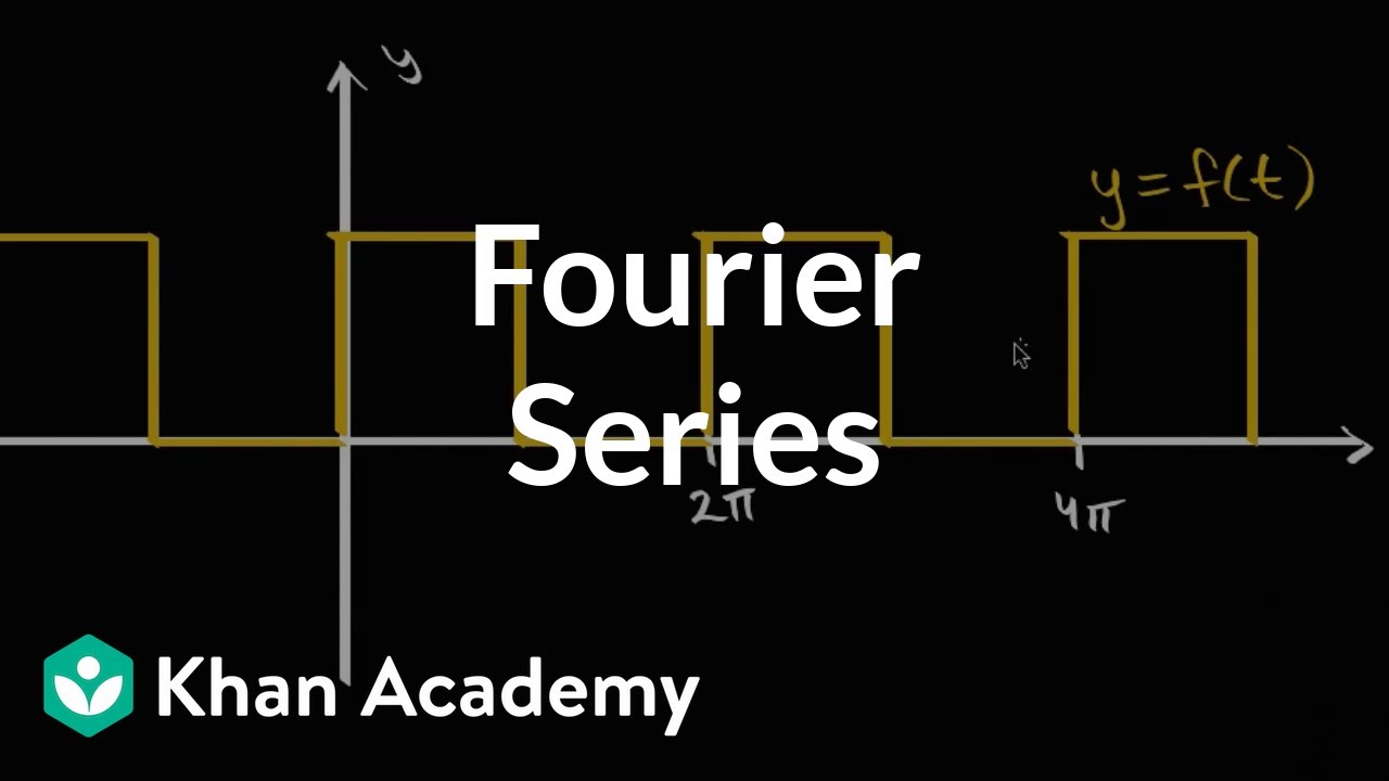 YouTube5:12
Another explanation of Fourier series.
Fourier seriesYouTube5:12Whiteboard for Fourier series, compared with the current visual explanation.
Fourier series