Read both sides of a graph near x=7, distinguish the limit 0 from g(7)=3, and identify a removable discontinuity.
Reviewed learning material · Video analysis · English
Read a graph where the curve has an open circle at (7,0) and a separate filled point at (7,3). The complete lesson approaches input 7 from both sides, finds nearby outputs tending to zero, then distinguishes the two-sided limit zero from the function value g(7)=3. The worked graph supplies local visual evidence and approximate samples, not an analytic formula or a formal epsilon-delta proof.
Generated from the video's visuals and explanation; not verbatim speech.
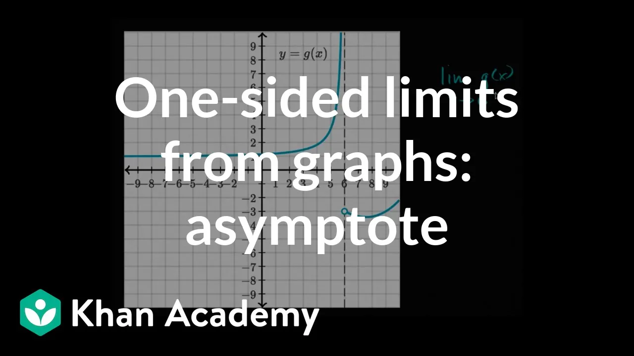
Inspect the graph y=g(x): an open circle lies at (7,0), while a separate filled point shares the input 7. The limit asks about nearby curve behavior, which can differ from the value at the point.
The speaker reframes the problem conceptually: instead of asking for the value exactly at x=7, the limit asks what output value the function approaches as the input values get closer and closer to 7. This sets up a graphical reading task rather than direct substitution.
To test that idea, the video begins with inputs less than 7. Pink dots are placed on the curve at x=3, 4, 5, 6, 6.5, 6.9, and 6.99, moving steadily rightward toward the vertical line x=7. The earlier outputs are only located visually, but the later ones are described more precisely: g(6) is a little less than -1, g(6.5) is around -0.5, and g(6.9) and g(6.99) are both below 0 but increasingly close to it.
For inputs sufficiently close to 7 from the left, the output approaches the open-circle height zero. The earlier samples need not all approach zero monotonically; they illustrate graph reading rather than a formal limit proof.
The board now shows the limit value zero. The lesson continues by checking the right side, which is also necessary for the two-sided conclusion.
The clip opens on a coordinate graph labeled y=g(x), with the handwritten statement \lim_{x \to 7} g(x)=0 already visible on the right. The mathematical task is to infer the limiting behavior at x=7 directly from the picture.
The narrator begins by choosing inputs larger than 7 and moving them closer to 7: first x=9, then x=8, then x=7.5, x=7.1, x=7.01, and finally x=7.0000001. Each choice is read off the graph, and the corresponding outputs are seen to shrink toward the x-axis.
The right-side samples supply a candidate right-hand limit zero. Combined with the preceding left-side observation, this supports the displayed two-sided graph estimate; finite samples alone are not a formal proof.
The next step changes the question from “what value is approached?” to “what value is actually assigned at the point?” A new handwritten line is added: g(7)=3. On the graph, this corresponds to the filled blue point located at (7,3), separate from the curve's approach level y=0.
Now the two quantities can be compared directly. The limit says the nearby outputs tend to 0, but the function value at the exact input 7 is 3. Since 0 \neq 3, the graph has an isolated break at that x-value.
The narrator names this break a point discontinuity, also called a removable discontinuity. Visually, that means the curve has a well-defined limiting height near x=7, but the plotted point has been displaced to a different height.
For an interior point c of a real function domain, continuity requires f(c) to be defined, a finite two-sided limit to exist, and that limit to equal f(c). In the displayed example the limit exists but differs from the assigned value, so continuity fails. Endpoint continuity uses the appropriate one-sided limit.
Knowledge cards
01
Limits
This segment introduces the problem of finding \lim_{x \to 7} g(x) from the graph of y=g(x). The graph contains a visible break at x=7: an open circle at (7,0) and a separate filled point above it. The narration explains that the limit question is about the value approached by the function as the inputs get closer to 7, not the isolated plotted value exactly at 7.
x→7limg(x)
02
Reading the left-hand approach
The inputs 3,4,5,6,6.5,6.9,6.99 increase toward the target 7. Farther samples need not move monotonically toward output zero: the curve initially drops and later rises. Sufficiently near the target, the left-side outputs approach the open-circle height.
03
Final written limit value
The first interval writes the value zero after inspecting the left side. The full lesson then checks the right side; agreeing one-sided limits support the two-sided result.
x→7limg(x)=0
04
Graphical estimation of a limit
The continuation samples inputs from the right. These outputs approach zero, agreeing with the preceding left-side investigation; both sides support the two-sided graph estimate.
x→7limg(x)=0
05
Right-side approach to x=7
The worked sequence uses x=9, 8, 7.5, 7.1, 7.01, and 7.0000001. As these x-values get nearer to 7 from above, the graph shows the y-values descending toward the x-axis, reinforcing the conclusion that the function approaches 0 near x=7.
06
Actual function value versus limiting value
The limit describes behavior near a point, while the function value describes what happens exactly at the point. Here the graph gives g(7)=3 from the filled point at (7,3), even though the surrounding curve approaches height 0. These are different kinds of information and should not be conflated.
g(7)=3,x→7limg(x)=0
07
Point discontinuity / removable discontinuity
In this example the finite two-sided limit is zero, but the assigned value is three. It is a removable discontinuity: redefining the value at the target to equal the limit would make the function continuous there. More generally, a removable discontinuity can also have no assigned value at the point.
x→7limg(x)=g(7)
08
Continuity test using limits
For an interior point c of a real function domain, continuity requires f(c) to be defined, a finite two-sided limit to exist, and that limit to equal f(c). In the displayed example the limit exists but differs from the assigned value, so continuity fails. Endpoint continuity uses the appropriate one-sided limit.
Check whether x→climf(x)=f(c).
Detailed learning notes
Explore conditions, steps and evidence. Supplementary explanations are labeled separately from content shown in the video.
Symbols · 10
y = g(x)
Clear evidence
Supplementary explanation
Evidence
Diagram
Observation
The graph is labeled y = g(x) on the left side of the coordinate plane.
Audio
Observation
The presenter introduces the graph of the function.
Symbol
y = g(x)
Meaning
The plotted function whose limit is being estimated from its graph.
Domain
The visible Cartesian window is approximately -9 to 9 on each axis; it is not a declaration of the full function domain.
\lim_{x \to 7} g(x)
Clear evidence
Shown in the video
Evidence
Formula
Observation
Yellow handwritten text on the right reads \lim_{x \to 7} g(x) =.
Audio
Observation
The presenter asks for the limit at the target input.
Symbol
\lim_{x \to 7} g(x)
Meaning
The two-sided limit of the function g(x) as the input x approaches 7.
Domain
The relevant inputs are values near x=7, not necessarily x=7 itself.
x \to 7
Clear evidence
Shown in the video
Evidence
Formula
Observation
The expression under the limit contains x \to 7.
Audio
Observation
The input is described as approaching the target.
Symbol
x \to 7
Meaning
The independent variable x is moving closer and closer to 7 from nearby values.
Domain
x is considered in a neighborhood of 7; the video emphasizes values less than 7.
g(x)
Clear evidence
Shown in the video
Evidence
Audio
Observation
The presenter samples the seven displayed inputs on the left.
Diagram
Observation
Pink dots mark corresponding output locations on the curve for those inputs.
Uncertainties
The exact numerical values of g(3), g(4), and g(5) are not written on screen; only their plotted positions are indicated.
Symbol
g(x)
Meaning
The output value of the function at a given input x, read vertically from the graph.
Domain
For the worked examples, x takes values 3, 4, 5, 6, 6.5, 6.9, and 6.99.
x=7
Clear evidence
Shown in the video
Evidence
Diagram
Observation
At x=7 there is an open circle on the curve at y=0 and a separate filled blue dot above it at approximately y=3.
Audio
Observation
The separated point is introduced as a point discontinuity.
Uncertainties
The exact y-coordinate of the isolated filled point is not labeled; it appears visually near 3.
Symbol
x=7
Meaning
The input value where the graph has a removable or point discontinuity and where the limit is being evaluated.
Domain
The discontinuity is shown at the vertical line x=7.
0
Clear evidence
Shown in the video
Evidence
Formula
Observation
A pink handwritten 0 is added after the equals sign, making \lim_{x \to 7} g(x) = 0.
Audio
Observation
The nearby output trend is described as approaching zero.
Symbol
0
Meaning
The estimated limiting output value of g(x) as x approaches 7 from the left-side sample sequence shown.
Domain
This is the y-value approached by the plotted outputs near x=7.
g(x)
Clear evidence
Supplementary explanation
Evidence
Formula
Observation
The graph is labeled y = g(x).
Audio
Observation
The presenter reads the right-side input samples and the target-point value.
Symbol
g(x)
Meaning
The function whose graph is used to estimate limiting behavior near x=7.
Domain
The visible graph window is approximately -9 to 9 in x; this is not a full domain specification. The lesson focuses near the target.
x \to 7
Clear evidence
Shown in the video
Evidence
Formula
Observation
The written expression is \lim_{x \to 7} g(x) = 0.
Audio
Observation
The nearby outputs are described as tending to zero.
Symbol
x \to 7
Meaning
The independent variable approaches the value 7; in this clip the emphasized numerical check is from values greater than 7.
Domain
Real-valued input near 7.
0
Clear evidence
Shown in the video
Evidence
Formula
Observation
The right-hand side of the limit statement is a pink handwritten 0.
Audio
Observation
Zero is identified as the approached output height.
Symbol
0
Meaning
The claimed limiting y-value of g(x) as x approaches 7.
Domain
Output value of g(x).
g(7)
Clear evidence
Shown in the video
Evidence
Formula
Observation
The handwritten expression becomes g(7) = 3.
Diagram
Observation
A filled blue point is shown at (7,3).
Audio
Observation
The assigned value at the target point is identified as three.
Symbol
g(7)
Meaning
The actual function value obtained by inputting x=7 into g.
Domain
Defined at x=7 in the displayed graph.
Knowledge points · 8
Estimating a limit from a graph
Clear evidence
Shown in the video
Evidence
Diagram
Observation
A coordinate graph labeled y=g(x) is shown with a discontinuity at x=7 and the prompt \lim_{x \to 7} g(x)= on the right.
Audio
Observation
The task is to estimate the displayed limit from the graph.
Method
Explanation
The video frames the problem as reading a limiting value from a plotted function rather than substituting the input into a formula. The key idea is to ask what output value the function approaches as the input gets closer to the target x-value.
Formula
Conditions
A graph of the function is available.
The target input value is identified on the x-axis.
The question concerns the behavior near the input, not necessarily the value at the input.
Point discontinuity shown on the graph
Clear evidence
Supplementary explanation
Evidence
Diagram
Observation
At x=7 the curve has an open circle at y=0 and a separate filled blue point above it.
Audio
Observation
The discontinuity at the target input is identified.
Uncertainties
The exact coordinate of the isolated filled point is not written; it is visually around (7,3).
Definition
Explanation
A point discontinuity is represented visually by a break in the curve at a single input. In this graph, the curve approaches one height near x=7, but the actual plotted point at x=7 is elsewhere, so the function value and the nearby trend do not match.
Formula
Conditions
The discontinuity occurs at a single x-value.
The graph shows nearby curve behavior plus an isolated or missing point at that x-value.
For the complete example, both one-sided limits agree at zero, while the filled point gives a different function value. A hole symbol alone does not establish a two-sided limit.
Prerequisites
Estimating a limit from a graph
Meaning of the limit notation in this example
Clear evidence
Shown in the video
Evidence
Audio
Observation
The presenter explains that a limit describes nearby output behavior.
Formula
Observation
The displayed expression is \lim_{x \to 7} g(x).
Definition
Explanation
The notation \lim_{x \to 7} g(x) is interpreted as the value that the outputs g(x) approach when the inputs x get closer and closer to 7. The explanation emphasizes approach rather than evaluation at x=7.
Formula
x→7limg(x)
Conditions
x is near 7.
The focus is on output behavior as inputs approach the target.
Prerequisites
Estimating a limit from a graph
Approaching the target from values less than 7
Clear evidence
Supplementary explanation
Evidence
Audio
Observation
The first approach uses input values below the target.
Diagram
Observation
Pink dots are placed successively on the curve at x=3, 4, 5, 6, 6.5, 6.9, and 6.99, moving rightward toward x=7.
Method
Explanation
The inputs 3,4,5,6,6.5,6.9,6.99 increase toward the target 7. Farther samples need not move monotonically toward output zero: the curve initially drops and later rises. Sufficiently near the target, the left-side outputs approach the open-circle height.
Formula
Conditions
Use input values less than 7.
Move the inputs progressively closer to 7.
Read the corresponding outputs from the graph.
This graph-reading lesson uses local behavior near the target. Finitely many samples illustrate the trend, not an epsilon-delta proof; no analytic formula is supplied.
Prerequisites
Meaning of the limit notation in this example
Point discontinuity shown on the graph
Graphical distinction between limiting height and actual point
Clear evidence
Supplementary explanation
Evidence
Diagram
Observation
The graph shows an open circle at (7,0) on the curve and a filled blue dot above it near (7,3).
Audio
Observation
The presenter focuses on nearby behavior rather than the isolated point.
Uncertainties
The exact y-coordinate of the filled point is not labeled; it appears close to 3.
Definition
Explanation
The open circle marks the height that the surrounding curve approaches at x=7, while the filled point marks the separately plotted function value at that input. The limit is read from the approach of nearby points, not from the isolated filled point.
Formula
Conditions
The graph contains both an open circle and a separate filled point at the same x-value.
The question asks for a limit rather than the function value at that x.
For the complete example, both one-sided limits agree at zero, while the filled point gives a different function value. A hole symbol alone does not establish a two-sided limit.
Prerequisites
Point discontinuity shown on the graph
Meaning of the limit notation in this example
Estimating a limit from a graph by approaching with sample inputs
Clear evidence
Supplementary explanation
Evidence
Audio
Observation
The presenter samples inputs from the right and reads approximate curve heights.
Diagram
Observation
Pink guide marks and dashed horizontal references show the corresponding y-values getting closer to the x-axis.
Formula
Observation
The persistent written conclusion is \lim_{x \to 7} g(x)=0.
Uncertainties
The exact decimal count in the spoken value after 7.01 is heard as 7.0000001, but the tiny visual difference near x=7 cannot be independently measured from the graph.
Method
Explanation
The clip demonstrates a graphical limit procedure: choose input values on one side of the target x-value, read the corresponding output values from the curve, and observe whether those outputs settle toward a single number. Here the chosen inputs are all greater than 7 and move closer to 7, so the method is being used to infer the limiting behavior near x=7 from the right.
Formula
x→7limg(x)=0
Conditions
The target point is x=7.
The displayed numerical check uses x>7.
The conclusion is read from the graph rather than from an algebraic formula for g.
This graph-reading lesson uses local behavior near the target. Finitely many samples illustrate the trend, not an epsilon-delta proof; no analytic formula is supplied.
This continuation checks the right side; the preceding interval checked the left. A two-sided finite limit requires both one-sided limits to exist and agree.
Point discontinuity / removable discontinuity at x=7
Clear evidence
Supplementary explanation
Evidence
Audio
Observation
The mismatch is named a point or removable discontinuity.
Diagram
Observation
The surrounding curve approaches the open circle at (7,0); the filled point at (7,3) gives the assigned value.
Formula
Observation
The board contrasts \lim_{x \to 7} g(x)=0 with g(7)=3.
Definition
Explanation
In this example the finite two-sided limit is zero, but the assigned value is three. It is a removable discontinuity: redefining the value at the target to equal the limit would make the function continuous there. More generally, a removable discontinuity can also have no assigned value at the point.
Formula
x→7limg(x)=g(7),0=3
Conditions
The limit exists at the point under discussion.
The function is defined at the point.
The limit value and function value are unequal.
Prerequisites
Estimating a limit from a graph by approaching with sample inputs
Continuity check by comparing limit and function value
Clear evidence
Supplementary explanation
Evidence
Audio
Observation
The presenter introduces comparison of a limit with the assigned value as a continuity check.
Formula
Observation
The comparison made on screen is between \lim_{x \to 7} g(x)=0 and g(7)=3.
Uncertainties
The video presents this as one way to test continuity and does not spell out the full formal definition with all standard clauses.
Method
Explanation
For an interior point c of a real function domain, continuity requires f(c) to be defined, a finite two-sided limit to exist, and that limit to equal f(c). In the displayed example the limit exists but differs from the assigned value, so continuity fails. Endpoint continuity uses the appropriate one-sided limit.
Formula
Check whether x→climf(x)=f(c).
Conditions
Applied at a specific input c.
Used here to detect discontinuity when the two quantities differ.
The video does not expand the full formal continuity definition beyond this comparison.
The complete formal clauses and endpoint qualification are editorial clarification; the source briefly introduces the comparison.
Prerequisites
Estimating a limit from a graph by approaching with sample inputs
Point discontinuity / removable discontinuity at x=7
Claims and conditions · 5
As x approaches 7 from below, g(x) approaches 0
Clear evidence
Shown in the video
Evidence
Audio
Observation
The presenter describes the local left-hand output trend toward zero.
Diagram
Observation
The pink sample points move along the curve toward the open circle at (7,0).
Formula
Observation
The final written result is \lim_{x \to 7} g(x)=0.
Uncertainties
This first interval explicitly develops only the left-side approach before ending; the written conclusion is presented as the limit value.
Proposition
Statement
For inputs approaching 7 from values less than 7, the plotted outputs of g(x) approach 0.
Hypotheses
The graph shown is y=g(x).
The inputs considered are less than 7 and get closer to 7.
Quantifiers
For x values approaching 7 from the left side.
The limit shown on screen equals 0
Clear evidence
Shown in the video
Evidence
Formula
Observation
The handwritten equation is completed as \lim_{x \to 7} g(x)=0.
Audio
Observation
The approaching output is identified as zero.
Uncertainties
This first interval ends immediately after writing the result; no separate right-side verification is shown within this segment.
Proposition
Statement
\lim_{x \to 7} g(x)=0.
Hypotheses
The graph is the one displayed in the video.
The limit is taken as x approaches 7.
Quantifiers
At the specific point x=7 for the function g.
Limit of g(x) as x approaches 7 is 0
Clear evidence
Shown in the video
Evidence
Formula
Observation
The written statement on screen is \lim_{x \to 7} g(x)=0.
Audio
Observation
The right-side output trend is described as approaching zero.
Diagram
Observation
Successive sample points with x>7 have y-values visually closer to the x-axis.
Uncertainties
The right-side investigation is shown in this interval; the left-side investigation appears in the preceding interval of the same full video.
Proposition
Statement
\lim_{x \to 7} g(x)=0
Hypotheses
The function is represented by the displayed graph y=g(x).
The target input value is x=7.
The numerical exploration shown in this clip uses x>7.
Quantifiers
For x tending to 7, the output values of g(x) tend to 0.
Actual function value at x=7 is 3
Clear evidence
Shown in the video
Evidence
Formula
Observation
The handwritten equation becomes g(7)=3.
Diagram
Observation
A filled blue point is plotted at (7,3).
Audio
Observation
The presenter reads the assigned value from the filled point.
Proposition
Statement
g(7)=3
Hypotheses
The graph defines the value of g at x=7.
The filled point at (7,3) represents the function value.
Quantifiers
At the single input x=7, the function takes the value 3.
Mismatch between limit and function value implies discontinuity at x=7
Clear evidence
Shown in the video
Evidence
Audio
Observation
The presenter identifies the mismatch as a removable discontinuity in this example.
Formula
Observation
The board shows both \lim_{x \to 7} g(x)=0 and g(7)=3.
Diagram
Observation
The surrounding curve approaches height zero, while the filled point at the target has height three.
Proposition
Statement
Because \lim_{x \to 7} g(x)=0 while g(7)=3, the function has a point discontinuity at x=7.
Hypotheses
The limit at x=7 exists and equals 0.
The function value at x=7 exists and equals 3.
0 \neq 3.
Quantifiers
At x=7, the limiting behavior and the assigned function value differ.
Derivations and proofs · 3
Reading the left-hand approach to the limit from sample inputs
Clear evidence
Supplementary explanation
Evidence
Audio
Observation
The presenter reads the seven displayed left-side input samples in order.
Diagram
Observation
Pink dots appear sequentially on the curve, and dashed pink guide lines indicate output levels near -1, -0.5, and just below 0.
Uncertainties
Exact values for g(3), g(4), and g(5) are not written; they are only located on the graph.
Individual verbal sample wording is uncertain; the positive near-target inputs are identified by their visible positions, not by an inferred negative-input example.
Visual argument
Steps
Expression
x=3
Explanation
The first sample input is chosen below 7 and marked on the curve.
Justification
The speaker begins with values less than 7 and identifies g(3) on the graph.
Shown in the video
Expression
x=4
Explanation
This input is closer to the target, but its curve height is lower than the preceding sample; output monotonicity over all listed samples is not required.
Justification
The native graph shows the far-left branch descending before turning upward.
Supplementary explanation
Expression
x=5
Explanation
The sample point moves still closer to 7.
Justification
The speaker names g(5) as another input approaching the target from below.
Shown in the video
Expression
x=6
Explanation
The output is read as a little less than -1.
Justification
The speaker says g(6) looks like it is a little bit less than negative 1, and a dashed guide line marks that level.
Shown in the video
Expression
x=6.5
Explanation
The output rises toward about -0.5.
Justification
The speaker says g(6.5) looks like it is around negative half, with another dashed guide line.
Shown in the video
Expression
x=6.9
Explanation
The output is now just below 0.
Justification
The speaker says the value looks a little bit less than zero as the input gets closer to 7.
Shown in the video
Expression
x=6.99
Explanation
The output remains below 0 but is even closer to 0.
Justification
The speaker says it is still less than zero but a little bit closer to zero.
Shown in the video
Expression
x→7−limg(x)=0
Explanation
The left-side sampled outputs approach the open-circle height at y=0.
Justification
Derived from the visible sequence of points converging to (7,0); the video writes the two-sided limit result immediately after this left-side discussion.
Derived from the video
Expression
x→7limg(x)=0
Explanation
The on-screen answer is completed as 0.
Justification
The written answer is visible before the first interval ends. A separate right-side check follows in the second interval of the full video.
Shown in the video
Conclusion
The first interval illustrates the left-side trend and records the proposed two-sided result; the continuation checks the other side. The result is a graph estimate rather than a proof from a supplied formula.
Deriving the limiting value 0 from right-side sample inputs
Clear evidence
Supplementary explanation
Evidence
Audio
Observation
The presenter works through the six right-side input samples in order.
Diagram
Observation
The corresponding graph positions move downward toward the x-axis as x moves leftward toward 7.
Formula
Observation
The written conclusion is \lim_{x \to 7} g(x)=0.
Uncertainties
The intermediate spoken estimates such as around 6, a little more than 2, and a little more than 1 are approximate readings from the graph, not exact computed values.
Intuitive argument
Steps
Expression
x=9⇒g(9) is about 6
Explanation
The narrator begins with a value clearly to the right of 7 and reads a relatively high output from the graph.
Justification
Direct reading from the displayed curve at x=9.
Shown in the video
Expression
x=8⇒g(8)>2
Explanation
Moving closer to 7, the output drops substantially.
Justification
Direct reading from the displayed curve at x=8.
Shown in the video
Expression
x=7.5⇒g(7.5)>1
Explanation
A still closer input gives an even smaller positive output.
Justification
Direct reading from the displayed curve at x=7.5.
Shown in the video
Expression
x=7.1⇒g(7.1)>0
Explanation
As x gets very close to 7 from above, the graph is just above the x-axis.
Justification
Direct reading from the displayed curve at x=7.1.
Shown in the video
Expression
x=7.01⇒g(7.01) is even closer to 0
Explanation
Reducing the distance to 7 further makes the output approach 0 more tightly.
Justification
Direct reading from the displayed curve at x=7.01.
Shown in the video
Expression
x=7.0000001⇒g(7.0000001) is still closer to 0
Explanation
An extremely close right-side input is used to reinforce the trend toward 0.
Justification
Spoken numerical example plus visual trend on the graph.
Shown in the video
Expression
x→7limg(x)=0
Explanation
The sequence of right-side outputs suggests the function values converge to 0 as x approaches 7.
Justification
This right-side graph estimate agrees with the left-side estimate in the preceding interval. Finite samples illustrate the trend rather than prove a general limit.
Supplementary explanation
Conclusion
From the displayed right-side approach, the graph indicates that g(x) tends to 0 as x approaches 7.
Concluding discontinuity from unequal limit and function value
Clear evidence
Shown in the video
Evidence
Audio
Observation
The approached value is compared with the assigned point value.
Formula
Observation
The board contains \lim_{x \to 7} g(x)=0 and later g(7)=3.
Diagram
Observation
The filled point at (7,3) is separated from the curve's approach level y=0.
Intuitive argument
Steps
Expression
x→7limg(x)=0
Explanation
First establish the limiting value from the graph.
Justification
Previously derived from approaching x=7 with nearby inputs.
Shown in the video
Expression
g(7)=3
Explanation
Then read the actual assigned value of the function at x=7 from the isolated point.
Justification
Direct reading from the filled point on the graph.
Shown in the video
Expression
0=3
Explanation
Compare the two quantities and note that they are not equal.
Justification
Arithmetic inequality of the displayed values.
Shown in the video
Expression
point discontinuity at x=7
Explanation
Because the limit and function value differ, the graph has a break at that input.
Justification
Continuity test stated by the narrator: if the limit is not the same as the actual value, there is a discontinuity.
Shown in the video
Conclusion
The function is discontinuous at x=7, specifically a point or removable discontinuity.
Worked examples · 2
Finding \lim_{x \to 7} g(x) from a graph with a point discontinuity
Clear evidence
Supplementary explanation
Evidence
Diagram
Observation
A graph of y=g(x) with a point discontinuity at x=7 is used throughout.
Formula
Observation
The prompt is \lim_{x \to 7} g(x)= and the completed answer is \lim_{x \to 7} g(x)=0.
Audio
Observation
Nearby inputs below the target are sampled to interpret the graph.
Uncertainties
This first interval ends at the transition to the right-side check, which is included in the full-video continuation.
Problem
Given the graph of y=g(x) with a discontinuity at x=7, determine the limit of g(x) as x approaches 7.
Given
The graph is labeled y=g(x).
There is a point discontinuity at x=7.
An open circle appears at (7,0).
A separate filled point appears above x=7, near y=3.
Goal
Determine \lim_{x \to 7} g(x).
Steps
Expression
Identify the target input x=7
Explanation
Locate the x-value where the limit is requested and observe the discontinuity there.
Justification
The speaker explicitly points out the discontinuity at x=7.
Shown in the video
Expression
Interpret x→7limg(x)
Explanation
Reframe the question as asking what output value the function approaches as inputs get near 7.
Justification
The speaker states that the function is being approached as the inputs approach 7.
Shown in the video
Expression
x=3,4,5,6,6.5,6.9,6.99
Explanation
Choose sample inputs less than 7 and move them closer and closer to 7.
Justification
The speaker begins with values less than 7 and lists these inputs in order.
Shown in the video
Expression
g(6)<−1,g(6.5)≈−0.5,g(6.9)<0,g(6.99)<0 and closer to 0
Explanation
These approximate local readings approach zero; earlier, more distant outputs need not do so monotonically.
Justification
These readings are spoken aloud and marked with pink dots and dashed guide lines.
Supplementary explanation
Expression
x→7limg(x)=0
Explanation
Conclude that the limiting output value is 0 and write it after the equals sign.
Justification
The speaker says the function value is approaching zero, and the final handwritten equation shows 0.
Shown in the video
Answer
0
Verification
The left-side samples illustrate approach to the open circle; the subsequent interval verifies the right side. Both are needed for the displayed two-sided answer.
Worked graphical example: limit versus function value at x=7
Clear evidence
Supplementary explanation
Evidence
Diagram
Observation
A single worked graph y=g(x) is used throughout the clip.
Audio
Observation
The nearby samples are compared with the value at the target input.
Formula
Observation
The final written facts are \lim_{x \to 7} g(x)=0 and g(7)=3.
Uncertainties
No algebraic formula for g(x) is provided, so the example is purely graphical.
Problem
Use the graph of y=g(x) to determine what happens to g(x) as x approaches 7, then compare that limiting behavior with the actual value g(7).
Given
The graph y=g(x) is displayed on a coordinate grid.
The target input is x=7.
Sample inputs shown in the narration include 9, 8, 7.5, 7.1, 7.01, and 7.0000001.
A filled point is plotted at (7,3).
Goal
Find \lim_{x \to 7} g(x), find g(7), and interpret whether the function is continuous at x=7.
Steps
Expression
x=9,8,7.5,7.1,7.01,7.0000001
Explanation
Choose inputs greater than 7 that move progressively closer to 7.
Justification
This is the sampling method used in the clip to inspect limiting behavior from the right.
Shown in the video
Expression
g(9)≈6,g(8)>2,g(7.5)>1,g(7.1)>0,g(7.01) closer to 0,g(7.0000001) even closer to 0
Explanation
Read the corresponding outputs from the graph and observe that they decrease toward the x-axis.
Justification
Direct graphical reading plus the narrator's spoken approximations.
Shown in the video
Expression
x→7limg(x)=0
Explanation
Infer the limiting value from the trend of the sampled outputs.
Justification
Combine the preceding left-side estimate with this right-side estimate; both approach the same height.
Supplementary explanation
Expression
g(7)=3
Explanation
Read the actual function value at x=7 from the isolated filled point.
Justification
Direct reading from the graph.
Shown in the video
Expression
x→7limg(x)=g(7)
Explanation
Compare the limit and the function value and note the mismatch.
Justification
Since 0 \neq 3, the two quantities differ.
Shown in the video
Expression
point discontinuity / removable discontinuity at x=7
Explanation
Classify the break using the continuity test mentioned in the narration.
Justification
The narrator states that differing limit and function value indicate discontinuity.
Shown in the video
Answer
\lim_{x \to 7} g(x)=0,\quad g(7)=3,\quad \text{so }g\text{ has a point (removable) discontinuity at }x=7.
Verification
The conclusion is checked against the graph: the curve approaches height 0 near x=7, while the separately marked filled point sits at height 3.
Visual events · 5
Initial setup of the graphical limit problem
Clear evidence
Shown in the video
Evidence
Diagram
Observation
The screen shows a Cartesian grid with the curve y=g(x), an open circle at (7,0), a filled blue point above x=7, and yellow text \lim_{x \to 7} g(x)= on the right.
Audio
Observation
The graph and the requested limit are introduced.
Uncertainties
The exact y-coordinate of the filled point is not labeled; it appears near 3.
Objects
Coordinate axes with grid lines
Curve labeled y=g(x)
Open circle at (7,0)
Filled blue point near (7,3)
Handwritten prompt \lim_{x \to 7} g(x)=
Changes
The cursor points first to the discontinuity at x=7 and then to the limit expression.
Invariants
The graph and prompt remain on screen throughout the setup.
The open circle stays at y=0 while the isolated filled point remains above it.
Interpretation
The visual setup establishes that the question is about the height approached by the curve near x=7, not the isolated plotted point at x=7.
Sequential marking of inputs approaching 7 from the left
Clear evidence
Supplementary explanation
Evidence
Animation
Observation
Pink dots are added one by one on the curve at x=3, 4, 5, 6, 6.5, 6.9, and 6.99.
Diagram
Observation
Dashed pink horizontal guide lines appear near y=-1 and y=-0.5 as the later sample points are discussed.
Audio
Observation
The presenter narrates the sampled inputs and approximate graph readings.
Uncertainties
The precise coordinates of the earliest sample points are not written on screen.
Objects
Pink sample dots on the curve
Dashed pink guide lines
x-axis labels 3 through 7
open circle at (7,0)
Changes
Sample points progress rightward toward x=7.
Farther outputs first decrease, then near-target outputs rise toward zero.
Guide lines emphasize that g(6) is a little less than -1 and g(6.5) is around -0.5.
Invariants
All highlighted sample inputs remain less than 7 during this sequence.
The target open circle at (7,0) does not move.
Interpretation
The inputs move right toward the target from below. Their near-target output trend approaches zero; the entire displayed sequence need not be monotonic.
Completion of the limit expression
Clear evidence
Shown in the video
Evidence
Formula
Observation
A pink handwritten 0 is added after the equals sign in \lim_{x \to 7} g(x)=.
Audio
Observation
The nearby values are described as approaching zero.
Uncertainties
No separate right-side approach is shown before the first interval ends.
Objects
Handwritten equation \lim_{x \to 7} g(x)=0
Graph with open circle at (7,0)
Changes
The blank after the equals sign is filled with 0.
Invariants
The graph remains unchanged while the answer is written.
Interpretation
The written 0 records the limiting height inferred from the nearby curve behavior at x=7.
Initial display of the graph and the limit statement
Clear evidence
Shown in the video
Evidence
Diagram
Observation
The left half shows a coordinate plane with y=g(x); the right half shows \lim_{x \to 7} g(x)=0 in handwriting.
Animation
Observation
Pink markers and dashed horizontal guides appear near x=7 to indicate output levels approaching the x-axis.
Uncertainties
The exact coordinates of every intermediate pink marker are not labeled numerically on screen.
Objects
Coordinate axes with integer gridlines
Blue curve labeled y=g(x)
Filled blue point at (7,3)
Handwritten limit statement \lim_{x \to 7} g(x)=0
Pink guide marks and dashed horizontal lines
Changes
Pink reference marks are added near x=7 to show output levels for sample inputs greater than 7.
The visual emphasis moves from larger x-values toward x=7, with corresponding y-levels descending toward 0.
Invariants
The underlying graph y=g(x) remains fixed.
The written limit statement remains \lim_{x \to 7} g(x)=0 during this interval.
Interpretation
The animation supports the idea that as x approaches 7 from the right, the function values approach 0.
Writing the actual function value g(7)=3
Clear evidence
Shown in the video
Evidence
Animation
Observation
A new handwritten line appears above the limit statement and is completed as g(7)=3.
Diagram
Observation
The cursor points to the filled blue point at (7,3) while the equation is being written.
Objects
Handwritten expression g(7)=3
Filled blue point at (7,3)
Existing limit statement \lim_{x \to 7} g(x)=0
Changes
The board adds g(7)=3 above the earlier limit statement.
Attention shifts from the limiting trend to the isolated defined point at x=7.
Invariants
The graph itself does not change.
The previously written limit value 0 remains visible.
Interpretation
This visual step sets up the direct comparison between the limit and the actual function value, revealing the discontinuity.
Misconceptions · 4
Confusing the limit with the actual function value at the discontinuity
Clear evidence
Derived from the video
Evidence
Diagram
Observation
The graph shows an open circle at (7,0) and a separate filled point above x=7.
Audio
Observation
The presenter investigates nearby outputs rather than substituting the target input.
Uncertainties
This clarification is analyst-derived from the contrast visible in the graph, not stated as an explicit warning in the first interval.
Misconception
One may think the limit at x=7 should equal the y-value of the isolated filled point shown at x=7.
Clarification
In this example the limit is read from the surrounding curve approaching the open circle at y=0, while the filled point represents a separate function value at the discontinuity.
Trying to evaluate the limit by direct substitution at a point discontinuity
Clear evidence
Derived from the video
Evidence
Audio
Observation
The task concerns the output trend near the target.
Animation
Observation
The solution proceeds by sampling nearby x-values instead of evaluating exactly at x=7.
Uncertainties
This is an analyst-derived teaching point based on the method shown in the video.
Misconception
One may expect to find the limit simply by plugging in x=7.
Clarification
The video instead determines the limit by observing the trend of g(x) for inputs near 7, which is necessary because the point at x=7 is disconnected from the nearby curve.
Do not confuse the limit with the function value at the point
Clear evidence
Shown in the video
Evidence
Audio
Observation
The presenter explicitly distinguishes the limit from the function value.
Formula
Observation
The board contrasts \lim_{x \to 7} g(x)=0 with g(7)=3.
Misconception
A common mistake is to assume that \lim_{x \to c} f(x) must equal f(c).
Clarification
This example shows they can differ: the limit is 0, but the actual value at x=7 is 3. That difference is exactly why the function is discontinuous there.
Terminology: point discontinuity versus removable discontinuity
Approximate timing
Shown in the video
Evidence
Audio
Observation
The presenter supplies point-discontinuity and removable-discontinuity names.
Uncertainties
The clip names the discontinuity type but does not explain the formal criterion that makes it removable beyond the displayed mismatch.
Misconception
Students may treat 'point discontinuity' and 'removable discontinuity' as unrelated terms.
Clarification
In this video they are presented as alternative names for the same kind of isolated break where the limit exists but differs from the assigned function value.
Concept relations · 7
Point discontinuity shown on the graph → Estimating a limit from a graph
Clear evidence
Shown in the video
Evidence
Diagram
Observation
The limit question is posed directly on a graph with a visible discontinuity at x=7.
Audio
Observation
The discontinuity and the limit task share the target input.
Application
Explanation
The concept of a point discontinuity provides the situation in which the graphical limit method is applied.
Meaning of the limit notation in this example → Approaching the target from values less than 7
Clear evidence
Supplementary explanation
Evidence
Formula
Observation
The displayed notation is \lim_{x \to 7} g(x).
Audio
Observation
The notation is explained through approaching inputs and outputs.
Application
Explanation
The meaning of the limit notation motivates the method of sampling nearby inputs and observing the output trend.
Graphical distinction between limiting height and actual point → Point discontinuity shown on the graph
Clear evidence
Shown in the video
Evidence
Diagram
Observation
The open circle at (7,0) and the separate filled point above x=7 are both visible throughout.
Audio
Observation
The presenter distinguishes the isolated point from nearby curve behavior.
Uncertainties
The exact coordinate of the filled point is not labeled.
Contrast
Explanation
The graph contrasts the limiting height represented by the open circle with the isolated actual point representing the discontinuity.
Approaching the target from values less than 7 → Finding \lim_{x \to 7} g(x) from a graph with a point discontinuity
Clear evidence
Shown in the video
Evidence
Animation
Observation
The example proceeds by placing sample points at x=3,4,5,6,6.5,6.9,6.99.
Audio
Observation
The first samples are taken below the target input.
Application
Explanation
The worked example applies the left-side sampling method to estimate the limit from the graph.
Estimating a limit from a graph by approaching with sample inputs → Point discontinuity / removable discontinuity at x=7
Clear evidence
Supplementary explanation
Evidence
Audio
Observation
The graph estimate is used when comparing limit and assigned value.
Formula
Observation
The relation is made explicit by writing both \lim_{x \to 7} g(x)=0 and g(7)=3.
Application
Explanation
The estimated limit is one of the two quantities compared to identify the discontinuity; it does not mean a left-hand limit alone is sufficient.
Point discontinuity / removable discontinuity at x=7 → Continuity check by comparing limit and function value
Clear evidence
Supplementary explanation
Evidence
Audio
Observation
The worked example motivates a general continuity check.
Formula
Observation
The displayed unequal limit and point value illustrate failure of the continuity equality; the example is not a proof of a general theorem.
Special case
Explanation
The specific break at x=7 is an instance of the broader continuity criterion: equality of limit and function value is required for continuity.
Estimating a limit from a graph by approaching with sample inputs → Continuity check by comparing limit and function value
Clear evidence
Derived from the video
Evidence
Audio
Observation
The continuity check involves understanding a limit and a point value.
Uncertainties
This prerequisite relation is made explicit by the analyst from the structure of the test, not by a separate formal theorem statement in the clip.
Prerequisite
Explanation
Understanding how to read a limit from a graph is required before applying the continuity test that compares that limit to f(c).
Find an answer · 9
What does \lim_{x \to 7} g(x) mean in this graphical example?
Clear evidence
Shown in the video
Evidence
Audio
Observation
The limit asks about the output approached near the target.
Formula
Observation
The expression \lim_{x \to 7} g(x) is shown on screen.
Knowledge points
Meaning of the limit notation in this example
Estimating a limit from a graph
Why is the limit read from the open circle instead of the isolated filled point at x=7?
Clear evidence
Shown in the video
Evidence
Diagram
Observation
An open circle at (7,0) and a separate filled point above x=7 are both shown.
Audio
Observation
The point discontinuity is discussed while investigating nearby values.
Uncertainties
The exact y-coordinate of the filled point is not labeled.
Knowledge points
Graphical distinction between limiting height and actual point
Point discontinuity shown on the graph
Confusing the limit with the actual function value at the discontinuity
How do you estimate a limit from values less than the target input?
Clear evidence
Shown in the video
Evidence
Audio
Observation
The presenter selects inputs below and increasingly near the target.
Animation
Observation
Pink dots are added at x=3,4,5,6,6.5,6.9,6.99.
Knowledge points
Approaching the target from values less than 7
Reading the left-hand approach to the limit from sample inputs
Finding \lim_{x \to 7} g(x) from a graph with a point discontinuity
What is the final limit value written for this graph?
Clear evidence
Shown in the video
Evidence
Formula
Observation
The completed equation reads \lim_{x \to 7} g(x)=0.
Audio
Observation
The approaching output is identified as zero.
Uncertainties
This first interval ends without showing a separate right-side verification.
Knowledge points
The limit shown on screen equals 0
Finding \lim_{x \to 7} g(x) from a graph with a point discontinuity
Does this segment verify the limit from the right side as well?
Clear evidence
Shown in the video
Evidence
Audio
Observation
The presenter transitions to investigating the other side.
Uncertainties
The continuation is absent from the provided segment.
Knowledge points
Reading the left-hand approach to the limit from sample inputs
The limit shown on screen equals 0
How do you estimate a limit from a graph by plugging in nearby x-values?
Pink guide marks show the trend toward the x-axis.
Knowledge points
Estimating a limit from a graph by approaching with sample inputs
Why can the limit at a point be different from the function's value at that point?
Clear evidence
Shown in the video
Evidence
Formula
Observation
The board shows \lim_{x \to 7} g(x)=0 and g(7)=3.
Audio
Observation
The presenter distinguishes a nearby trend from the value at the point.
Knowledge points
Point discontinuity / removable discontinuity at x=7
Continuity check by comparing limit and function value
What does a point or removable discontinuity look like on a graph?
Clear evidence
Shown in the video
Evidence
Audio
Observation
The point/removable discontinuity is identified in the graph.
Diagram
Observation
An isolated filled point at (7,3) sits away from the curve's limiting height 0.
Knowledge points
Point discontinuity / removable discontinuity at x=7
How do you use limits to test whether a function is continuous at a point?
Clear evidence
Shown in the video
Evidence
Audio
Observation
The limit and assigned value are compared to check continuity.
Knowledge points
Continuity check by comparing limit and function value
Coverage and review notes
Covered · Introduction of the graph, the point discontinuity at x=7, and the limit question.
Covered · Step-by-step sampling of inputs less than 7 and reading the corresponding outputs from the graph.
Covered · The answer 0 is written after the limit expression, and the speaker begins to transition to checking values from the other side before the clip ends.
Covered · The clip uses sample inputs greater than 7 and graphical reading to argue that g(x) approaches 0 as x approaches 7.
Covered · The narrator writes g(7)=3, compares it with the limit 0, identifies a point/removable discontinuity, and states the continuity test.
This segment introduces the problem of finding \lim_{x \to 7} g(x) from the graph of y=g(x). The graph contains a visible break at x=7: an open circle at (7,0) and a separate filled point above it. The narration explains that the limit question is about the value approached by the function as the inputs get closer to 7, not the isolated plotted value exactly at 7.
 math
math