Reviewed learning material · Video analysis · EnglishRead the full overview
This 120-second introductory visual lesson explains a two-state Markov chain using weather. It defines the Markov property, builds a transition graph with Sunny and Rainy states, assigns probabilities 0.8, 0.2, 0.4, and 0.6, encodes them in the transition matrix P=[[0.8,0.2],[0.4,0.6]], then introduces the initial distribution π=[0.5,0.5] and updates it day by day via π=πP to show convergence toward a steady state.
This 23-second clip shows a two-state weather Markov chain with states Sunny and Rainy. A day counter advances from Day 5 to Day 8 while the displayed probabilities move from 66% / 34% to 67% / 33%, and the final frame annotates these as approximately 2/3 and 1/3. Throughout, the equation π=π⋅P remains on screen, identifying the limiting distribution as a steady state. The narration states that the probabilities settle toward specific values and that, for this example, the distribution converges to the same steady state regardless of where it started. The clip ends with an informal summary that this is basically how Markov chains work.
Use the learning inspector for key ideas and moments, or open the reading tabs for the complete notes.
Generated from the video's visuals and explanation; not verbatim speech.
The clip opens by posing a concrete prediction problem: if we know only today's weather, how can we estimate tomorrow's? Visually, the title "Markov Chains" appears, then two state nodes labeled Sunny and Rainy are introduced. This sets up a discrete-state probabilistic model rather than a deterministic forecast.
The narrator states the central idea: in these systems, the future depends only on the present, not the past. The on-screen phrase "Only today matters, not yesterday" reinforces the Markov property. At this point the mathematical object being built is a two-state stochastic process with state space {Sunny, Rainy}.
The lesson next specifies how the process moves in time. Each day the system transitions from one state to another, and the diagram explicitly allows self-loops. That means a sunny day may be followed by another sunny day, and similarly for rain. The four directed edges encode all possible one-step moves.
The key property is restated in probabilistic language: the distribution of tomorrow's state depends only on today's state. This is not merely a storytelling simplification; it is the defining assumption of a Markov chain. The graph therefore represents a memoryless one-step transition mechanism.
Numbers are then attached to the arrows. From Sunny, the probability of staying Sunny is 0.8 and the probability of switching to Rainy is 0.2. From Rainy, the probability of switching to Sunny is 0.4 and the probability of staying Rainy is 0.6. These are one-step transition probabilities.
Immediately after labeling the graph, the video checks normalization: 0.8+0.2=1 and 0.6+0.4=1. The reason is that from any current state, the system must end up in some next state. Thus the outgoing probabilities from each state form a probability distribution.
The same information is then repackaged algebraically as a transition matrix. With rows indexed by starting states and columns by ending states, the matrix is P=[[0.8,0.2],[0.4,0.6]]. The entry in row i, column j is the probability of moving from state i to state j in one step.
The row-sum condition is repeated in matrix form: each row of P sums to 1. This makes clear that the matrix is not an arbitrary array of numbers; it is a stochastic matrix encoding the full one-step dynamics of the two-state system.
To study evolution over time, the video adds an initial state distribution, denoted π. Here π=[0.5,0.5], meaning that at Day 0 there is a 50% chance of Sunny and a 50% chance of Rainy. This shifts attention from a single known starting state to a probability vector over states.
The update mechanism is then shown: each day the distribution is multiplied by the transition matrix, displayed as π=π⋅P. Interpreted iteratively, this means πn+1=πnP. The animation turns this abstract rule into visible change in the bar heights.
Starting from [0.5, 0.5], one multiplication gives Day 1: [0.6, 0.4]. Another gives Day 2: [0.64, 0.36]. A third gives Day 3: approximately [0.66, 0.34], with the exact value [0.656, 0.344] rounded on screen. The Sunny share rises while the Rainy share falls.
The final section is titled "Convergence to Steady State," and the changing bars illustrate that repeated application of P drives the distribution toward a limiting profile. The clip ends during this demonstration, so the trend is clear even though the exact steady-state vector is not explicitly completed within these 120 seconds.
The clip opens on a black slide titled “Convergence to Steady State.” Two colored state markers are already present: a yellow circle labeled Sunny and a blue circle labeled Rainy. Above them are two bars showing current probabilities, with the left label reading Day 5. At the bottom, the equation π=π⋅P is displayed continuously, signaling that the discussion concerns a fixed-point distribution for a Markov chain.
As the narrator says that something interesting happens, the animation advances the day counter. The visual emphasis is on change over discrete time steps: the distribution is being updated from one day to the next rather than treated as a static table of numbers.
Between Day 5 and Day 8, the Sunny percentage rises from 66% to 67%, while the Rainy percentage falls from 34% to 33%. The movement is small but systematic, and the bars stop changing appreciably at the displayed rounding precision. This is the concrete demonstration of convergence: repeated application of the transition rule drives the state probabilities toward stable values.
When the narrator says “Two thirds sunny, one third rainy,” the final frame adds explicit fractional annotations beside the bars: ≈32 for Sunny and ≈31 for Rainy. These annotations connect the rounded decimal percentages to the intended exact limiting proportions. The use of ≈ is important because 67% and 33% are rounded displays, not exact equalities.
The narration then states that no matter how many more days pass, and no matter where the process started, the distribution converges to the same steady state. Within this clip, that claim is supported by the example’s visible stabilization and by the persistent equation π=π⋅P. The equation says that once the distribution reaches π, applying the transition matrix P leaves it unchanged.
Mathematically, the example can be read as follows: if μn is the distribution on Day n, the animation suggests μ5=(0.66,0.34), then μ6=(0.67,0.33), and by Days 7 and 8 the displayed values remain (0.67,0.33), with the intended limit π≈(32,31). The clip does not show the matrix P itself, so the exact update rule cannot be reconstructed from this segment alone; what is shown is the outcome of iterating that rule.
The narrator closes with the informal summary, “And that’s basically how Markov chains work.” This should be understood as a pedagogical takeaway from the example, not as a fully general theorem. The segment demonstrates one important behavior—approach to a steady-state distribution—but it does not state the broader conditions under which every Markov chain has a unique limiting steady state.
In summary, the clip teaches three linked ideas in order: a two-state Markov chain example, day-by-day convergence of its probability distribution, and identification of the limit as a steady state satisfying π=π⋅P. The final visual message is that the long-run behavior can be simpler and more stable than the individual daily transitions.
Knowledge cards
01
Markov chain: memoryless stochastic system
Type: definition. A Markov chain is a system whose next state depends only on the current state, not on earlier history. The video introduces this through weather prediction and the on-screen phrase "Only today matters, not yesterday." Formula: none. Applicable to discrete-time processes with a well-defined state space. Prerequisites: basic probability. Related: Markov property, states, transitions. Evidence: 15-48s. To verify: none.
02
States in the weather example
Type: definition. The example uses two states, Sunny and Rainy, shown as two labeled nodes. Each day the system occupies one of these states before transitioning. Formula: state space = {Sunny, Rainy}. Prerequisites: none. Related: transitions, transition matrix. Evidence: 23-31s. To verify: none.
{Sunny,Rainy}
03
Transitions and self-loops
Type: definition. A transition is a one-step move from one state to another. The diagram includes self-loops, so the system may remain in the same state from one day to the next. Formula: none. Conditions: transitions are considered between consecutive time steps. Prerequisites: states. Related: transition probabilities. Evidence: 31-48s. To verify: none.
04
One-step transition probabilities
Type: formula. The graph assigns probabilities to each directed edge: from Sunny, 0.8 stay Sunny and 0.2 become Rainy; from Rainy, 0.4 become Sunny and 0.6 stay Rainy. Formula: p_{SS}=0.8, p_{SR}=0.2, p_{RS}=0.4, p_{RR}=0.6. Conditions: probabilities are nonnegative and describe one-step moves. Prerequisites: transitions. Related: row-sum property, transition matrix. Evidence: 48-70s. To verify: none.
pSS=0.8,pSR=0.2,pRS=0.4,pRR=0.6
05
Outgoing probabilities must sum to 1
Type: formula. Because the system must end up in some state after one step, the probabilities leaving each state add to 1. The video checks this numerically as 0.8+0.2=1 and 0.6+0.4=1. Formula: ∑jp_{ij}=1. Conditions: applies for each fixed starting state i. Prerequisites: transition probabilities. Related: transition matrix rows. Evidence: 65-70s. To verify: none.
j∑pij=1
06
Transition matrix of a two-state chain
Type: definition. The transition matrix stores all one-step probabilities, with rows as starting states and columns as ending states. For this example, P=[[0.8,0.2],[0.4,0.6]]. Formula: P=[0.80.40.20.6]. Conditions: each row sums to 1. Prerequisites: transition probabilities, state labels. Related: matrix indexing, distribution update. Evidence: 71-93s. To verify: none.
P=[0.80.40.20.6]
07
Meaning of matrix entry (i,j)
Type: definition. The entry in row i, column j gives the probability of moving from state i to state j in one step. In the displayed matrix, row S corresponds to starting Sunny and column R to ending Rainy, so the top-right entry 0.2 is P(Sunny today -> Rainy tomorrow). Formula: p_{ij}=P(Xt+1=j∣Xt=i). Conditions: uses the row-start / column-end convention stated in the video. Prerequisites: transition matrix. Related: transition probabilities. Evidence: 80-87s. To verify: none.
pij=P(Xt+1=j∣Xt=i)
08
Initial state distribution
Type: definition. Before evolving the chain over time, one specifies a probability distribution over the states at the starting time. The example takes complete uncertainty: 50% Sunny and 50% Rainy. Formula: π=[0.5,0.5]. Conditions: entries are nonnegative and sum to 1. Prerequisites: states. Related: distribution update. Evidence: 94-106s. To verify: none.
π=[0.5,0.5]
09
Updating the distribution with the transition matrix
Type: method. To advance one day, multiply the current distribution by the transition matrix. The video displays π=π⋅P and animates repeated updates from Day 0 to Day 3. Formula: πn+1=πnP (equivalently shown as π←πP). Conditions: use the same one-step transition matrix at each iteration. Prerequisites: transition matrix, initial distribution. Related: convergence to steady state. Evidence: 106-119s. To verify: the clip does not explicitly write time subscripts, though iteration is shown visually.
πn+1=πnP
10
Worked daily updates in the weather example
Type: example. Starting from π0=[0.5,0.5], repeated multiplication by P gives π1=[0.6,0.4], π2=[0.64,0.36], and π3=[0.656,0.344], rounded on screen to 66% and 34%. Formula: [0.5,0.5]P=[0.6,0.4]; [0.6,0.4]P=[0.64,0.36]; [0.64,0.36]P=[0.656,0.344]. Prerequisites: distribution update. Related: transition matrix, convergence. Evidence: 106-120s. To verify: none.
[0.5,0.5]P=[0.6,0.4]
11
Convergence toward a steady state
Type: method. The final animation shows the distribution changing less dramatically over time, illustrating approach to a steady-state profile under repeated multiplication by P. Formula: steady state satisfies π∗=π∗P. Conditions: the video presents this as an illustrative convergence behavior in this example. Prerequisites: distribution update. Related: transition matrix, long-run behavior. Evidence: 94-120s. To verify: the exact limiting vector is not explicitly completed before the clip ends.
π∗=π∗P
12
Common pitfall: forgetting self-loops
Type: misconception. Learners sometimes assume a Markov chain must change state at every step. The video explicitly draws self-loops and says a sunny day can be followed by another sunny day, so staying put is allowed with positive probability. Prerequisites: transitions. Related: transition probabilities. Evidence: 31-38s. To verify: none.
13
Common pitfall: swapping rows and columns in P
Type: misconception. The matrix convention can be confused. The video states that each row is a starting state and each column is an ending state, so entry (i,j) means i -> j, not j -> i. Prerequisites: transition matrix. Related: matrix indexing. Evidence: 75-87s. To verify: none.
14
Steady state equation for a Markov chain
The clip displays the fixed-point equation π=π⋅P throughout. Here π is the steady-state probability distribution and P is the transition matrix. The equation means that once the chain’s distribution reaches π, one more step of transitions leaves the distribution unchanged. In the example shown, this steady state corresponds approximately to (32,31) for Sunny and Rainy.
π=π⋅P
15
Two-state weather Markov chain example
The visual model has exactly two states, Sunny and Rainy, represented by colored circles and bars. A day counter advances from Day 5 to Day 8, showing how the probability distribution evolves over discrete time. This example is used to make the abstract idea of Markov-chain convergence concrete.
16
Observed convergence to 2/3 and 1/3
The displayed probabilities move from 66% Sunny and 34% Rainy on Day 5 to 67% Sunny and 33% Rainy by Day 8. The final frame annotates these as ≈32 and ≈31, indicating that the intended limiting distribution is two-thirds sunny and one-third rainy. The rounded percentages are visual approximations, while the fractions express the cleaner limiting values emphasized by the narration.
π≈(32,31)
17
Same steady state regardless of starting point in this example
The narrator states that no matter where the process started, the distribution converges to the same steady state. In this clip, that claim is illustrated by the stabilizing bars and the persistent fixed-point equation. It is presented as a feature of the example rather than proved as a general theorem for all Markov chains.
18
What this short clip does and does not prove
The segment provides a visual and verbal demonstration of convergence in a specific two-state Markov chain. It shows the limiting values and names the steady-state condition π=π⋅P. However, it does not display the transition matrix P, does not derive the fractions algebraically, and does not state the general hypotheses needed for uniqueness or convergence of arbitrary Markov chains.
Detailed learning notes
Explore conditions, steps and evidence. Supplementary explanations are labeled separately from content shown in the video.
Symbols · 8
P
Clear evidence
Shown in the video
Evidence
Formula
Observation
The screen shows the transition matrix labeled P=[[0.8,0.2],[0.4,0.6]].
Audio
Observation
The narrator says, "We can encode all this information in a transition matrix P."
Symbol
P
Meaning
Transition matrix of the two-state Markov chain; entry in row i, column j gives the probability of moving from state i to state j.
Domain
2x2 matrix with nonnegative entries and row sums equal to 1.
p_{ij}
Clear evidence
Shown in the video
Evidence
Audio
Observation
The narrator says, "The entry in row i, column j tells you the probability of going from state i to state j."
Formula
Observation
Matrix entries are displayed numerically as 0.8, 0.2, 0.4, 0.6.
Symbol
p_{ij}
Meaning
Probability of transitioning from starting state i to ending state j in one step.
Domain
For this example, i,j∈S,R; values shown are p_{SS}=0.8, p_{SR}=0.2, p_{RS}=0.4, p_{RR}=0.6.
S, R
Clear evidence
Shown in the video
Evidence
Formula
Observation
Column labels S and R appear above the matrix, and row labels S and R appear to its right.
Audio
Observation
The narrator says, "Each row represents a starting state, each column an ending state."
Symbol
S, R
Meaning
State labels for Sunny and Rainy used to index rows and columns of the transition matrix.
Domain
Discrete state set of the weather example.
π
Clear evidence
Shown in the video
Evidence
Formula
Observation
The screen shows π=[0.5,0.5].
Audio
Observation
The narrator says, "the initial state distribution, which we call pi."
Symbol
π
Meaning
Initial state distribution over the states Sunny and Rainy.
Domain
Row vector of probabilities summing to 1; here π=[0.5,0.5].
π=π⋅P
Clear evidence
Shown in the video
Evidence
Formula
Observation
The bottom formula changes to π=π⋅P.
Audio
Observation
The narrator says, "Each day, we apply the transition probabilities."
Uncertainties
The displayed equation uses the same symbol π on both sides, so it is visually ambiguous whether it denotes iterative update or fixed-point condition; the surrounding animation shows repeated updating day by day.
Symbol
π=π⋅P
Meaning
One-step update rule shown for evolving the state distribution under the transition matrix.
Domain
Applied iteratively in the animation from Day 0 onward.
π
Clear evidence
Shown in the video
Evidence
Formula
Observation
Bottom center shows the equation π=π⋅P.
Symbol
π
Meaning
Steady-state probability distribution vector; in the visual example it corresponds to the limiting probabilities for Sunny and Rainy.
Domain
Probability distribution over the Markov chain states
P
Clear evidence
Shown in the video
Evidence
Formula
Observation
Bottom center shows the equation π=π⋅P.
Uncertainties
The matrix P is not displayed explicitly in this clip; its entries are not visible here.
Symbol
P
Meaning
Transition matrix of the Markov chain.
Domain
Matrix whose rows describe transition probabilities between states
n in Day n
Clear evidence
Shown in the video
Evidence
Animation
Observation
Left label changes from Day 5 to Day 6, Day 7, and Day 8.
Symbol
n in Day n
Meaning
Discrete time index or day number used to track the evolving state distribution.
Domain
Positive integers
Knowledge points · 11
Definition of a Markov chain
Clear evidence
Shown in the video
Evidence
Audio
Observation
The narrator defines Markov chains as systems where the future depends only on the present, not the past.
Caption evidence
Observation
On-screen text reads "Only today matters, not yesterday".
Definition
Explanation
A Markov chain is a stochastic system whose next state depends only on the current state and not on earlier history. In the video this is introduced through the weather question: if today is sunny, what is the chance tomorrow is sunny?
Formula
Conditions
The process has discrete states.
The conditional distribution of the next state depends only on the present state.
Prerequisites
States of the weather model
States of the weather model
Clear evidence
Shown in the video
Evidence
Audio
Observation
The narrator says, "We start with states, in this case, sunny or rainy."
Diagram
Observation
Two circles labeled Sunny and Rainy appear on screen.
Definition
Explanation
The example uses two states, Sunny and Rainy. Each day the system occupies exactly one of these states before transitioning to the next day.
Formula
Conditions
State space in this example is {Sunny, Rainy}.
Transitions and self-loops
Clear evidence
Shown in the video
Evidence
Audio
Observation
The narrator says, "Each day, the weather transitions from one state to another. Notice that we can stay in the same state."
Animation
Observation
Self-loops are drawn on Sunny and Rainy, then arrows between the two states are added.
Caption evidence
Observation
Text appears: "Each arrow: possible transition".
Definition
Explanation
A transition is a move from one state to another in one time step. The diagram explicitly includes self-loops, showing that the system may remain in the same state from one day to the next.
Formula
Conditions
Transitions occur one step at a time.
Staying in the same state is allowed.
Prerequisites
States of the weather model
One-step transition probabilities
Clear evidence
Shown in the video
Evidence
Audio
Observation
The narrator assigns 80% stay sunny, 20% become rainy, 40% clear up, and 60% stay rainy.
Formula
Observation
Numbers 0.8, 0.2, 0.4, 0.6 appear on the arrows.
Formula
Observation
The screen shows 0.8+0.2=1 and later 0.6+0.4=1.
Formula
Explanation
Each outgoing arrow from a state carries a probability. From Sunny: 0.8 to remain Sunny and 0.2 to become Rainy. From Rainy: 0.4 to become Sunny and 0.6 to remain Rainy. The probabilities leaving each state must sum to 1.
Formula
pSS=0.8,pSR=0.2,pRS=0.4,pRR=0.6
Conditions
For each fixed starting state, the outgoing probabilities sum to 1.
Probabilities are nonnegative.
Prerequisites
Transitions and self-loops
Row-sum property of transition probabilities
Clear evidence
Shown in the video
Evidence
Audio
Observation
The narrator says, "Notice that the probabilities leaving each state must sum to 1. You have to end up somewhere."
Formula
Observation
The equations 0.8+0.2=1 and 0.6+0.4=1 are displayed.
Formula
Explanation
Because the system must move to some state after one step, the probabilities of all outcomes from a given current state add to 1. This is first shown on the graph and then restated for the matrix rows.
Formula
j∑pij=1
Conditions
Applies to each starting state i.
In this example the sums are 0.8+0.2=1 and 0.6+0.4=1.
Prerequisites
One-step transition probabilities
Transition matrix representation
Clear evidence
Shown in the video
Evidence
Audio
Observation
The narrator says, "We can encode all this information in a transition matrix P. Each row represents a starting state, each column an ending state."
Formula
Observation
The matrix P=[[0.8,0.2],[0.4,0.6]] is shown with row and column labels S and R.
Caption evidence
Observation
Text appears: "Each row sums to 1".
Definition
Explanation
The transition matrix collects all one-step transition probabilities. Row index denotes the current state and column index denotes the next state, so the (i,j) entry is the probability of going from state i to state j.
Formula
P=[0.80.40.20.6]
Conditions
Rows correspond to starting states.
Columns correspond to ending states.
Each row sums to 1.
Prerequisites
One-step transition probabilities
Row-sum property of transition probabilities
States of the weather model
Initial state distribution
Clear evidence
Shown in the video
Evidence
Audio
Observation
The narrator says, "Now, we need one more ingredient: the initial state distribution, which we call pi."
Formula
Observation
The screen shows π=[0.5,0.5].
Diagram
Observation
Two bars above Sunny and Rainy are labeled 50% and 50%.
Definition
Explanation
To study how the system evolves over time, one must specify the probability distribution over states at the starting time. The example chooses complete uncertainty: 50% Sunny and 50% Rainy.
Formula
π=[0.5,0.5]
Conditions
Entries are probabilities over the state space.
They sum to 1.
Prerequisites
States of the weather model
Updating the state distribution
Clear evidence
Shown in the video
Evidence
Audio
Observation
The narrator says, "What happens as we step forward in time? Each day, we apply the transition probabilities."
Formula
Observation
The displayed equation becomes π=π⋅P.
Animation
Observation
The bars change from 50%/50% to 60%/40%, then 64%/36%, then 66%/34%.
Uncertainties
The video does not explicitly write a time index such as πn+1=πnP; it shows the update rule in the compact form π=π⋅P while animating successive days.
Method
Explanation
The distribution over states is advanced one day at a time by multiplying the current distribution by the transition matrix. Repeated multiplication produces the sequence of bar heights shown in the animation.
Formula
π←πP
Conditions
Use the same transition matrix at each step.
The distribution is updated iteratively over time.
Prerequisites
Transition matrix representation
Initial state distribution
Steady state of a Markov chain
Clear evidence
Shown in the video
Evidence
Audio
Observation
Narrator says the probabilities settle toward specific values, two-thirds sunny and one-third rainy, and that the distribution converges to the same steady state.
Formula
Observation
Equation π=π⋅P is shown throughout.
Animation
Observation
Bars stabilize at 67% Sunny and 33% Rainy by Day 8, with approximations ≈ 2/3 and ≈ 1/3 appearing.
Definition
Explanation
A steady state is a probability distribution that remains unchanged after applying the transition rule of the Markov chain. In this clip it is represented by the fixed point equation π=π⋅P and visually by the limiting proportions 2/3 for Sunny and 1/3 for Rainy.
Formula
π=π⋅P
Conditions
The object is a probability distribution over the states of a Markov chain.
The distribution is being compared before and after multiplication by the transition matrix P.
Prerequisites
Two-state weather Markov chain example
Two-state weather Markov chain example
Clear evidence
Shown in the video
Evidence
Audio
Observation
Narrator concludes, "And that's basically how Markov chains work."
Diagram
Observation
Two labeled states appear as circles: Sunny and Rainy.
Animation
Observation
Day counter advances while the two state probabilities change and then stabilize.
Uncertainties
The transition probabilities defining P are not shown in this clip.
Method
Explanation
The clip uses a two-state weather model with states Sunny and Rainy to illustrate how repeated transitions drive an initial distribution toward a limiting distribution. The method shown is to iterate the state probabilities day by day and observe convergence.
Conditions
There are two states, Sunny and Rainy.
The process is discrete-time, indexed by days.
Convergence of the day-by-day distribution
Clear evidence
Shown in the video
Evidence
Audio
Observation
Narrator says, "No matter how many more days pass, and no matter where we started, the distribution converges to the same steady state."
Animation
Observation
Sunny rises from 66% to 67%, Rainy falls from 34% to 33%, and the fractions ≈ 2/3 and ≈ 1/3 appear beside the bars.
Uncertainties
The clip does not prove convergence; it demonstrates it numerically and visually for this example.
Formula
Explanation
As the day index increases, the probability distribution over states approaches a limiting vector. In this example the limiting proportions are approximately 2/3 for Sunny and 1/3 for Rainy, matching the steady-state interpretation of π=π⋅P.
Formula
n→∞limμn=π,π≈(32,31)
Conditions
μn denotes the distribution on Day n.
The displayed limit is for the specific two-state example shown in the video.
Prerequisites
Steady state of a Markov chain
Two-state weather Markov chain example
Claims and conditions · 5
Markov property
Clear evidence
Shown in the video
Evidence
Audio
Observation
The narrator says, "The key property of a Markov chain is this: the probability of tomorrow's state depends only on today's state, not on yesterday."
Caption evidence
Observation
Earlier on-screen text states "Only today matters, not yesterday".
Proposition
Statement
For a Markov chain, the probability distribution of the next state depends only on the current state, not on earlier states.
Hypotheses
The system is a Markov chain.
States are observed at successive discrete times.
Quantifiers
For each current state, the conditional distribution of the next state is independent of the past history.
Total probability from each state
Clear evidence
Shown in the video
Evidence
Audio
Observation
The narrator says, "Notice that the probabilities leaving each state must sum to 1. You have to end up somewhere."
Formula
Observation
The equations 0.8+0.2=1 and 0.6+0.4=1 are shown.
Proposition
Statement
The probabilities of all possible one-step transitions leaving a given state sum to 1.
Hypotheses
The transition probabilities are properly defined for one time step.
The system must occupy some state after the step.
Quantifiers
For every starting state i, the sum over all ending states j equals 1.
Transition matrix captures the dynamics
Clear evidence
Shown in the video
Evidence
Audio
Observation
The narrator says, "This matrix captures the complete structure of the system."
Formula
Observation
The full matrix P=[[0.8,0.2],[0.4,0.6]] is displayed with row and column labels.
Uncertainties
The statement is true for the one-step transition structure of this finite Markov chain; the video does not discuss additional structure such as periodicity or reducibility.
Proposition
Statement
The transition matrix encodes the complete one-step structure of the Markov chain example.
Hypotheses
The system's dynamics are fully described by one-step transition probabilities between the listed states.
Quantifiers
For this two-state example, all one-step transition probabilities are contained in P.
Same steady state regardless of starting distribution
Clear evidence
Shown in the video
Evidence
Audio
Observation
Narrator says, "no matter where we started, the distribution converges to the same steady state."
Uncertainties
This statement is presented for the example in the clip; the video does not state the general hypotheses under which all Markov chains have this property.
Proposition
Statement
For the Markov chain example shown, the distribution converges to the same steady state no matter where the process started.
Hypotheses
The process is the two-state Markov chain illustrated in the clip.
The transition dynamics remain the same across days.
Quantifiers
For the example shown, for any starting distribution mentioned by the narrator.
Informal summary of Markov chain behavior
Clear evidence
Shown in the video
Evidence
Audio
Observation
Narrator says, "And that's basically how Markov chains work."
Uncertainties
This is an informal summary statement rather than a precise theorem.
Proposition
Statement
The clip presents convergence to a steady state as the basic behavior of Markov chains.
Hypotheses
The discussion refers to the two-state weather example just shown.
Quantifiers
Informal, based on the example in this clip.
Derivations and proofs · 7
Verification that outgoing probabilities sum to one
Clear evidence
Shown in the video
Evidence
Formula
Observation
The screen displays 0.8+0.2=1 and then 0.6+0.4=1.
Audio
Observation
The narrator explains that probabilities leaving each state must sum to 1.
Numerical verification
Steps
Expression
0.8+0.2=1
Explanation
From the Sunny state, the two outgoing probabilities are 0.8 to stay Sunny and 0.2 to become Rainy.
Justification
Direct reading of the labeled arrows on the graph.
Shown in the video
Expression
0.6+0.4=1
Explanation
From the Rainy state, the two outgoing probabilities are 0.6 to stay Rainy and 0.4 to become Sunny.
Justification
Direct reading of the labeled arrows on the graph.
Shown in the video
Conclusion
Each state's outgoing transition probabilities total 1, matching the requirement that the system must end up in some state after one step.
Day 0 to Day 1 distribution update
Clear evidence
Derived from the video
Evidence
Formula
Observation
The screen shows π=[0.5,0.5] and then the update rule π=π⋅P.
Animation
Observation
Day 1 bars read 60% Sunny and 40% Rainy.
Uncertainties
The intermediate arithmetic is not spoken aloud; it is inferred from the displayed initial vector, matrix, and resulting Day 1 percentages.
Numerical verification
Steps
Expression
π0=[0.5,0.5]
Explanation
The initial distribution assigns equal probability to Sunny and Rainy.
Justification
Displayed formula and bar labels at Day 0.
Shown in the video
Expression
π1=π0P=[0.5,0.5][0.80.40.20.6]
Explanation
Apply the transition matrix once to advance one day.
Justification
Shown update rule π=π⋅P together with the matrix definition.
After three steps the exact distribution is [0.656,0.344], rounded on screen to 66% Sunny and 34% Rainy.
Trend toward a steady state
Approximate timing
Derived from the video
Evidence
Animation
Observation
The sequence of distributions moves 50/50 -> 60/40 -> 64/36 -> 66/34 under repeated multiplication by P.
Formula
Observation
The section title is "Convergence to Steady State".
Uncertainties
The clip ends before the limiting value is stated explicitly, so the steady-state numbers are inferred from the displayed trend and standard fixed-point calculation rather than directly spoken in this segment.
Intuitive argument
Steps
Expression
πn+1=πnP
Explanation
Repeatedly applying the transition matrix updates the distribution day by day.
Justification
Displayed update rule and animated sequence of daily distributions.
Derived from the video
Expression
50%→60%→64%→66% for Sunny
Explanation
The Sunny probability increases while the Rainy probability decreases, suggesting approach to a limit.
Justification
Observed bar heights across Day 0 to Day 3.
Shown in the video
Expression
π∗=π∗P
Explanation
A steady-state distribution would remain unchanged after one more multiplication by P.
Justification
Standard fixed-point interpretation of the displayed convergence section title.
Supplementary explanation
Conclusion
The animation illustrates convergence toward a steady-state distribution, though the exact limiting vector is not explicitly completed within this 120-second clip.
Visual derivation of convergence in the example
Clear evidence
Shown in the video
Evidence
Animation
Observation
Day 5 shows 66% Sunny and 34% Rainy; Day 6 shows 67% and 33%; Day 7 shows 67% and 33%; Day 8 shows 67% and 33% with ≈ 2/3 and ≈ 1/3 added.
Audio
Observation
Narrator explains that the probabilities settle toward specific values and converge to the same steady state.
Uncertainties
The exact transition matrix is not shown, so the numerical update rule cannot be reconstructed from this clip alone.
Visual argument
Steps
Expression
Day 5:(0.66,0.34)
Explanation
The animation begins with the distribution on Day 5, assigning 66% to Sunny and 34% to Rainy.
Justification
Directly read from the on-screen labels and bar heights.
Shown in the video
Expression
Day 6:(0.67,0.33)
Explanation
After one more day, the Sunny probability increases slightly and the Rainy probability decreases slightly.
Justification
Directly read from the updated on-screen labels.
Shown in the video
Expression
Day 7:(0.67,0.33)
Explanation
The displayed rounded percentages remain the same on Day 7, indicating stabilization at the shown precision.
Justification
Directly read from the on-screen labels.
Shown in the video
Expression
Day 8:(0.67,0.33),0.67≈32,0.33≈31
Explanation
By Day 8 the video adds fractional approximations beside the bars, identifying the stable values with 2/3 and 1/3.
Justification
Directly read from the added text ≈ 2/3 and ≈ 1/3.
Shown in the video
Expression
π=π⋅P
Explanation
The persistent bottom equation interprets the stable pair as a fixed point of the transition operation.
Justification
Formula shown on screen throughout the clip.
Shown in the video
Conclusion
The example visually demonstrates that repeated transitions drive the distribution toward the steady-state values approximately (2/3, 1/3).
Editorial check that (2/3, 1/3) sums to 1
Clear evidence
Supplementary explanation
Evidence
Formula
Observation
On-screen approximations show 0.67 ≈ 2/3 and 0.33 ≈ 1/3.
Formula
Observation
The steady-state equation π=π⋅P is shown.
Uncertainties
This step is supplied by the analyst to explain why the displayed fractions are consistent; the video itself does not perform the algebra.
Intuitive argument
Steps
Expression
32+31=1
Explanation
The two limiting probabilities add to one, so they can represent a valid probability distribution over the two states.
Justification
Basic arithmetic of fractions.
Supplementary explanation
Expression
π≈(32,31)
Explanation
Thus the displayed steady-state vector is consistent with a normalized two-state distribution.
Justification
Combines the on-screen approximations with the normalization check.
Supplementary explanation
Conclusion
The displayed limiting values are internally consistent as a probability distribution.
Worked examples · 2
Weather Markov chain example
Clear evidence
Shown in the video
Evidence
Audio
Observation
The entire clip uses the weather example with Sunny and Rainy states and specified transition probabilities.
Diagram
Observation
A two-node graph and then a 2x2 matrix are built from the example.
Animation
Observation
Daily distributions are updated from the initial vector [0.5,0.5].
Problem
Model tomorrow's weather using only today's weather, with states Sunny and Rainy and given transition probabilities.
Given
States: Sunny, Rainy.
From Sunny: 0.8 stay Sunny, 0.2 become Rainy.
From Rainy: 0.4 become Sunny, 0.6 stay Rainy.
Initial distribution: π=[0.5,0.5].
Goal
Represent the process as a Markov chain, encode it in a transition matrix, and update the state distribution over several days.
Steps
Expression
States ={Sunny,Rainy}
Explanation
Identify the state space of the model.
Justification
Stated directly in the narration and shown as two labeled nodes.
Shown in the video
Expression
P=[0.80.40.20.6]
Explanation
Place the one-step transition probabilities into a matrix with rows as starting states and columns as ending states.
Justification
Explicitly constructed on screen and explained by the narrator.
Shown in the video
Expression
π0=[0.5,0.5]
Explanation
Choose an initial distribution reflecting complete uncertainty about today's weather.
Justification
Displayed formula and 50%/50% bars at Day 0.
Shown in the video
Expression
π1=[0.6,0.4],π2=[0.64,0.36],π3≈[0.66,0.34]
Explanation
Update the distribution repeatedly by multiplying by P to obtain the next day's probabilities.
Justification
Animation shows these values; the arithmetic follows from πn+1=πnP.
Derived from the video
Answer
The example yields the transition matrix P=[[0.8,0.2],[0.4,0.6]] and the evolving distributions [0.5,0.5] -> [0.6,0.4] -> [0.64,0.36] -> approximately [0.66,0.34].
Verification
Each row of P sums to 1, and the displayed daily bar percentages match the results of successive multiplication by P.
Weather Markov chain convergence example
Clear evidence
Shown in the video
Evidence
Diagram
Observation
States are labeled Sunny and Rainy.
Animation
Observation
Day counter advances from Day 5 to Day 8 while percentages update.
Audio
Observation
Narrator describes settling to two-thirds sunny and one-third rainy.
Uncertainties
Initial distribution before Day 5 is not shown in this clip.
Transition matrix P is not shown in this clip.
Problem
Track the day-by-day probabilities for a two-state weather model with states Sunny and Rainy and identify the limiting distribution.
Given
State set: {Sunny, Rainy}.
Day 5 distribution shown as 66% Sunny and 34% Rainy.
Subsequent displayed days are Day 6, Day 7, and Day 8.
Steady-state relation shown as π=π⋅P.
Goal
Determine what values the probabilities approach as days increase.
Steps
Expression
Start from Day 5: (0.66,0.34)
Explanation
Read the initial displayed distribution for the example.
Justification
Visible on screen at the beginning of the clip.
Shown in the video
Expression
Update through Day 6–8
Explanation
Advance the day counter and observe the new percentages for Sunny and Rainy.
Justification
Animation shows successive day labels and updated bar values.
Shown in the video
Expression
(0.67,0.33)≈(32,31)
Explanation
The stabilized rounded percentages are identified with the fractions shown beside the bars.
Justification
On-screen text adds ≈ 2/3 and ≈ 1/3 by Day 8.
Shown in the video
Answer
The distribution converges to approximately 2/3 Sunny and 1/3 Rainy.
Verification
The narrator explicitly states the limiting values, and the final frame displays 67% ≈ 2/3 and 33% ≈ 1/3 alongside the steady-state equation.
Visual events · 7
Introduction of the two-state weather setup
Clear evidence
Shown in the video
Evidence
Animation
Observation
The title "Markov Chains" appears, followed by two circular nodes labeled Sunny and Rainy.
Caption evidence
Observation
Text appears: "What's tomorrow's weather?" and then "Only today matters, not yesterday".
Objects
Title text "Markov Chains"
Sunny node
Rainy node
Question text
Memoryless-property text
Changes
Title appears first.
Two state nodes are introduced.
Question text appears below the nodes.
Text emphasizing dependence only on today appears.
Invariants
There are exactly two states in the example.
The state labels remain Sunny and Rainy.
Interpretation
The opening visual frames the lesson as a probabilistic prediction problem with a two-state system and highlights the Markov memoryless property.
Construction of the transition diagram
Clear evidence
Shown in the video
Evidence
Animation
Observation
A self-loop is drawn on Sunny, then an arrow from Sunny to Rainy, then a self-loop on Rainy, then an arrow from Rainy to Sunny.
Caption evidence
Observation
Text reads "Each arrow: possible transition".
Objects
Sunny node
Rainy node
Self-loop on Sunny
Arrow Sunny to Rainy
Self-loop on Rainy
Arrow Rainy to Sunny
Caption text
Changes
Arrows are added one by one until all four possible one-step transitions are present.
Invariants
The two state nodes stay fixed in place.
All transitions are one-step possibilities between the same two states.
Interpretation
The diagram shows that from either state the system can either remain in place or switch to the other state, giving four possible directed transitions.
Assignment of transition probabilities
Clear evidence
Shown in the video
Evidence
Animation
Observation
Numeric labels 0.8, 0.2, 0.4, and 0.6 appear on the corresponding arrows.
Formula
Observation
Equations 0.8+0.2=1 and 0.6+0.4=1 appear beneath the graph.
Objects
Four directed arrows
Numeric probability labels
Sum-to-one equations
Changes
Each arrow receives a probability value.
Row-wise sums are displayed to verify normalization.
Invariants
The underlying graph structure does not change while probabilities are added.
Interpretation
The visual converts the qualitative transition graph into a quantitative Markov chain by attaching probabilities and checking that outgoing mass from each state totals 1.
Encoding the graph as a matrix
Clear evidence
Shown in the video
Evidence
Animation
Observation
The title changes to "The Transition Matrix" and a 2x2 matrix is built entry by entry.
Formula
Observation
Labels S and R appear above columns and beside rows; the final matrix is [[0.8,0.2],[0.4,0.6]].
Caption evidence
Observation
Text reads "Each row sums to 1".
Objects
Transition graph
Matrix brackets
Entries 0.8, 0.2, 0.4, 0.6
Row labels S,R
Column labels S,R
Caption text
Changes
Graph information is transferred into matrix form.
Row and column labels are added to clarify indexing.
The row-sum statement is displayed.
Invariants
The numerical transition probabilities remain the same as on the graph.
Interpretation
The matrix presentation makes explicit that rows index current states and columns index next states, turning the diagram into a compact algebraic object.
Evolution of the state distribution over time
Clear evidence
Shown in the video
Evidence
Animation
Observation
Bars above Sunny and Rainy appear at Day 0 with 50% and 50%, then update to Day 1 60%/40%, Day 2 64%/36%, Day 3 66%/34%.
Formula
Observation
The formula π=[0.5,0.5] is shown and later replaced by π=π⋅P.
Uncertainties
The exact frame-by-frame interpolation between day labels is not fully resolved, but the displayed day labels and percentages are clear.
Objects
Day label
Sunny bar
Rainy bar
Percentage labels
Initial distribution formula
Update formula
Changes
The day counter advances from Day 0 to Day 3.
The Sunny bar grows while the Rainy bar shrinks.
The formula shifts from a static initial vector to an update rule.
Invariants
The two bars always represent probabilities over the same two states.
Their heights continue to sum to 100%.
Interpretation
The animation demonstrates how repeated multiplication by the transition matrix moves the probability distribution toward a more Sunny-heavy profile, illustrating convergence behavior.
Day-by-day probability animation
Clear evidence
Shown in the video
Evidence
Animation
Observation
Left label changes from Day 5 to Day 6, Day 7, and Day 8 while the yellow and blue bars update.
Diagram
Observation
Yellow circle labeled Sunny and blue circle labeled Rainy remain fixed below the bars.
Objects
Title "Convergence to Steady State"
Left day label
Yellow Sunny bar
Blue Rainy bar
Yellow Sunny circle
Blue Rainy circle
Bottom equation π=π⋅P
Fraction annotations ≈ 2/3 and ≈ 1/3 appearing later
Changes
Day label advances from Day 5 to Day 8.
Sunny percentage changes from 66% to 67%.
Rainy percentage changes from 34% to 33%.
Fraction annotations ≈ 2/3 and ≈ 1/3 appear beside the bars by Day 8.
Invariants
The two state labels Sunny and Rainy remain on screen.
The equation π=π⋅P remains visible throughout.
The color coding stays consistent: yellow for Sunny, blue for Rainy.
Interpretation
The animation illustrates iterative evolution of a probability distribution until it reaches a stable limiting profile.
Persistent steady-state equation
Clear evidence
Shown in the video
Evidence
Formula
Observation
Bottom center continuously shows π=π⋅P.
Objects
Equation π=π⋅P
Invariants
The equation remains unchanged for the full clip.
Interpretation
The formula identifies the limiting distribution as a fixed point of right-multiplication by the transition matrix.
Misconceptions · 7
Confusing Markov dependence with full-history dependence
Clear evidence
Shown in the video
Evidence
Audio
Observation
The narrator contrasts "only on the present, not the past" and later repeats "not on yesterday."
Caption evidence
Observation
On-screen text says "Only today matters, not yesterday".
Misconception
One might think tomorrow's weather could depend on a longer sequence of past days.
Clarification
The video explicitly states the defining Markov property: the probability of tomorrow's state depends only on today's state, not on yesterday or earlier history.
Assuming transitions must change the state
Clear evidence
Shown in the video
Evidence
Audio
Observation
The narrator says, "Notice that we can stay in the same state. A sunny day can be followed by another sunny day."
Animation
Observation
Self-loops are drawn on both Sunny and Rainy.
Misconception
A learner may think a Markov chain must move to a different state at every step.
Clarification
The diagram includes self-loops, showing that remaining in the same state is a valid transition with positive probability.
Swapping the roles of rows and columns in the transition matrix
Clear evidence
Shown in the video
Evidence
Audio
Observation
The narrator says, "Each row represents a starting state, each column an ending state."
Formula
Observation
Row and column labels S and R are displayed around the matrix.
Misconception
One may mistakenly read columns as starting states and rows as ending states.
Clarification
The video defines the convention clearly: row index is the current state and column index is the next state, so entry (i,j) is the probability of going from i to j.
Thinking any matrix direction could sum to 1
Clear evidence
Shown in the video
Evidence
Audio
Observation
The narrator says the probabilities leaving each state must sum to 1 and later says each row sums to 1.
Formula
Observation
The displayed checks are 0.8+0.2=1 and 0.6+0.4=1, followed by the caption "Each row sums to 1".
Misconception
A learner might assume columns, not rows, should sum to 1.
Clarification
In this convention, the normalization condition applies to rows because each row lists all possible destinations from a fixed starting state.
Confusing the chain itself with a known starting state
Clear evidence
Shown in the video
Evidence
Audio
Observation
The narrator introduces the initial state distribution and says, "Let's say we're completely uncertain about today's weather: 50% sunny, 50% rainy."
Formula
Observation
The screen shows π=[0.5,0.5].
Misconception
One may think a Markov chain analysis begins only when the current state is known with certainty.
Clarification
The video shows that one can instead begin with a probability distribution over states, here 50/50, and then evolve that distribution over time.
Do not confuse rounded percentages with exact fractions
Clear evidence
Supplementary explanation
Evidence
Animation
Observation
The bars display 67% and 33%, while separate annotations show ≈ 2/3 and ≈ 1/3.
Misconception
Seeing 67% and 33% may lead a viewer to treat those decimals as the exact steady-state values.
Clarification
The video distinguishes the rounded percentages from the approximate fractions by writing ≈ 2/3 and ≈ 1/3, indicating that the exact limiting values being suggested are 2/3 and 1/3 rather than the rounded decimals themselves.
Example convergence is not a full general theorem statement
Clear evidence
Supplementary explanation
Evidence
Audio
Observation
Narrator says convergence happens no matter where we started, but only for the example being discussed.
Diagram
Observation
Only a two-state weather example is shown.
Misconception
One might infer from this short clip that every Markov chain necessarily converges to a unique steady state.
Clarification
This segment demonstrates convergence in a specific two-state example and states the steady-state equation, but it does not provide the general conditions required for all Markov chains.
Concept relations · 11
States of the weather model → Transitions and self-loops
Clear evidence
Shown in the video
Evidence
Audio
Observation
The narration first introduces states and then says each day the weather transitions from one state to another.
Animation
Observation
Nodes appear before arrows are added.
Prerequisite
Explanation
Transitions are defined only after the state space is introduced; the graph arrows connect previously named states.
Transitions and self-loops → One-step transition probabilities
Clear evidence
Shown in the video
Evidence
Animation
Observation
Probability numbers are placed onto already drawn arrows.
Audio
Observation
The narrator says, "Let's add numbers" after describing possible transitions.
Prerequisite
Explanation
Quantitative transition probabilities are attached to the qualitative transition structure already shown in the graph.
One-step transition probabilities → Row-sum property of transition probabilities
Clear evidence
Shown in the video
Evidence
Formula
Observation
The sums 0.8+0.2=1 and 0.6+0.4=1 are written directly from the displayed outgoing probabilities.
Audio
Observation
The narrator explains the sums immediately after assigning the probabilities.
Contains
Explanation
The row-sum condition is a direct property of the set of outgoing transition probabilities from each state.
The narrator says the transition matrix encodes all this information.
Formula
Observation
The matrix entries match the arrow labels exactly.
Equivalent
Explanation
For this finite example, the labeled transition graph and the matrix P contain the same one-step probabilistic information.
Definition of a Markov chain → Markov property
Clear evidence
Shown in the video
Evidence
Audio
Observation
The definition of Markov chains and the later statement of the key property both emphasize dependence only on the present state.
Proof dependency
Explanation
The defining feature of the Markov chain concept in this clip is exactly the Markov property stated as a proposition.
Transition matrix representation → Updating the state distribution
Clear evidence
Shown in the video
Evidence
Formula
Observation
The matrix P is introduced before the update rule π=π⋅P appears.
Animation
Observation
Daily distribution changes are produced after the matrix has been defined.
Application
Explanation
The transition matrix is the operator used to advance the state distribution from one day to the next.
Initial state distribution → Updating the state distribution
Clear evidence
Shown in the video
Evidence
Formula
Observation
The initial vector π=[0.5,0.5] is shown before the update rule and the animated daily changes.
Audio
Observation
The narrator introduces the initial distribution and then asks what happens stepping forward in time.
Prerequisite
Explanation
A starting distribution is needed before one can iterate the update rule and observe convergence over time.
Updating the state distribution → Trend toward a steady state
Approximate timing
Derived from the video
Evidence
Animation
Observation
Repeated updates produce a visibly stabilizing sequence of percentages.
Caption evidence
Observation
The section title is "Convergence to Steady State".
Uncertainties
The exact steady-state value is not completed within the clip, so the relation is to the convergence idea rather than a fully stated theorem.
Application
Explanation
Iterating the distribution update is what produces the apparent convergence toward a steady state illustrated in the final section.
Two-state weather Markov chain example → Steady state of a Markov chain
Clear evidence
Shown in the video
Evidence
Audio
Observation
Narrator links the weather example to the phrase "the same steady state" and then to "how Markov chains work."
Formula
Observation
π=π⋅P is displayed beneath the weather-state graphic.
Application
Explanation
The two-state weather example is used to apply and illustrate the abstract steady-state definition π=π⋅P.
Steady state of a Markov chain → Convergence of the day-by-day distribution
Clear evidence
Shown in the video
Evidence
Audio
Observation
Narrator first says the probabilities settle toward specific values and then names the limit a steady state.
Animation
Observation
The day-by-day bars approach the values later annotated as ≈ 2/3 and ≈ 1/3.
Special case
Explanation
The convergence statement is the dynamic realization of the steady-state idea in this example: the iterated distribution approaches the fixed point π.
Convergence of the day-by-day distribution → Same steady state regardless of starting distribution
Clear evidence
Shown in the video
Evidence
Audio
Observation
Narrator says convergence occurs no matter where we started.
Proof dependency
Explanation
The claim about independence of the starting point depends on the observed convergence behavior of the distribution in the example.
Find an answer · 11
What does it mean that a Markov chain depends only on the present and not the past?
Clear evidence
Shown in the video
Evidence
Audio
Observation
The narrator defines Markov chains and states the key property.
Caption evidence
Observation
Text emphasizes "Only today matters, not yesterday".
Knowledge points
Definition of a Markov chain
Markov property
How are states and transitions represented in a simple two-state weather Markov chain?
Clear evidence
Shown in the video
Evidence
Audio
Observation
The narrator introduces states and transitions, including staying in the same state.
Animation
Observation
Self-loops and cross-arrows are drawn between Sunny and Rainy.
Knowledge points
States of the weather model
Transitions and self-loops
Why must the probabilities leaving each state sum to 1, and how does that appear in the transition matrix?
Clear evidence
Shown in the video
Evidence
Formula
Observation
The sums 0.8+0.2=1 and 0.6+0.4=1 are shown, followed by "Each row sums to 1".
Audio
Observation
The narrator explains why outgoing probabilities must total 1.
Knowledge points
One-step transition probabilities
Row-sum property of transition probabilities
Transition matrix representation
Total probability from each state
In the transition matrix, which index is the current state and which is the next state?
Clear evidence
Shown in the video
Evidence
Audio
Observation
The narrator says rows are starting states and columns are ending states.
Formula
Observation
The matrix is labeled with S and R on both axes.
Knowledge points
Transition matrix representation
P
p_{ij}
S, R
What is the initial state distribution and why is it needed before evolving the chain?
Clear evidence
Shown in the video
Evidence
Formula
Observation
The screen shows π=[0.5,0.5].
Audio
Observation
The narrator calls this the initial state distribution.
Knowledge points
Initial state distribution
π
How do you update a state distribution from one day to the next using the transition matrix?
Clear evidence
Shown in the video
Evidence
Formula
Observation
The displayed rule is π=π⋅P.
Animation
Observation
Day-by-day bar changes follow repeated application of this rule.
Uncertainties
The clip does not explicitly introduce time subscripts, though the animation clearly shows iteration.
Knowledge points
Updating the state distribution
π=π⋅P
Day 0 to Day 1 distribution update
Day 1 to Day 2 distribution update
Day 2 to Day 3 distribution update
What does the animation suggest about convergence to a steady state in this Markov chain?
Approximate timing
Shown in the video
Evidence
Caption evidence
Observation
The section title reads "Convergence to Steady State".
Animation
Observation
The distribution sequence approaches a more stable split across days.
Uncertainties
The exact limiting distribution is not stated before the clip ends.
Knowledge points
Trend toward a steady state
Evolution of the state distribution over time
What does the equation π=π⋅P mean for a Markov chain?
Clear evidence
Supplementary explanation
Evidence
Formula
Observation
π=π⋅P is shown on screen.
Audio
Observation
Narrator refers to the same steady state.
Knowledge points
Steady state of a Markov chain
Convergence of the day-by-day distribution
Why does the video say the limiting probabilities are two-thirds sunny and one-third rainy?
Clear evidence
Supplementary explanation
Evidence
Animation
Observation
Final frame shows 67% ≈ 2/3 and 33% ≈ 1/3.
Audio
Observation
Narrator says two-thirds sunny, one-third rainy.
Knowledge points
Convergence of the day-by-day distribution
Weather Markov chain convergence example
Does the steady state depend on the initial distribution in this example?
Clear evidence
Supplementary explanation
Evidence
Audio
Observation
Narrator says no matter where we started, the distribution converges to the same steady state.
Knowledge points
Same steady state regardless of starting distribution
Convergence of the day-by-day distribution
What basic Markov chain behavior is illustrated by this clip?
Clear evidence
Supplementary explanation
Evidence
Audio
Observation
Narrator concludes, "And that's basically how Markov chains work."
Knowledge points
Two-state weather Markov chain example
Steady state of a Markov chain
Convergence of the day-by-day distribution
Coverage and review notes
Covered · Opening motivation: predicting tomorrow's weather from today's weather introduces the Markov setting and the two states.
Covered · The memoryless property is stated verbally and on screen, and the Sunny/Rainy state space is established.
Covered · Transition diagram is built with self-loops and cross-arrows, showing possible one-step moves.
Covered · Numerical probabilities are attached to arrows and checked by summing outgoing probabilities from each state.
Covered · The graph is encoded as a 2x2 transition matrix with row/column labels and the row-sum property restated.
Covered · The initial distribution π=[0.5,0.5] is introduced with matching 50%/50% bars.
Covered · The update rule π=πP is shown and iterated through Day 1, Day 2, and Day 3, illustrating movement toward a steady state.
Covered · The entire clip is a single continuous visual explanation of convergence to a steady state in a two-state Markov chain example, accompanied by narration and the persistent equation π=π⋅P.