Compare two nearly normal score distributions: means60 and65, standard deviations10 and5. Read centers, spread and peak height to identify diagram A.
Reviewed learning material · Video analysis · English
A score-distribution question separates the location and shape of normal curves. School A has mean60 and standard deviation10; School B has mean65 and standard deviation5. The thick line represents School A, and the thin line School B. School A must have a leftward center and a wider, lower peak; School B a rightward center and a narrower, higher peak. The complete source selects diagram A. The question describes real scores as close to normal, so the comparison uses a normal model. The area-1 intuition applies to the same normalized normal family on the same coordinate scale, not to arbitrary densities merely sharing area 1.
Generated from the video's visuals and explanation; not verbatim speech.
Identify the lines first: thick for School A, thin for School B. The scores are close to normal; we compare normal models without requiring an exactly normal empirical sample.
Use the mean for location and the standard deviation for shape. The mean is the symmetry center of a normal curve; on the same axes its standard deviation controls horizontal scale and peak height.
School A has mean60, below School B’s65, so the thick curve’s center is left of the thin curve’s center. This compares centers; it does not mean the curves have disjoint support.
School A’s standard deviation10 exceeds School B’s5. Its normal curve is wider with a lower peak; School B’s is narrower with a higher peak. Check width and height as well as the centers.
Both normal densities have total area 1. Horizontal stretching of the same normal family lowers density height by the reciprocal scale. The editorial peak formula is f(μ)=1/(σ2π): the entire product of the standard deviation and the square root of 2π is in the denominator. Diagram B’s equal peaks fail this comparison, and the source selects A. A density height is not the probability of a single score.
Combine the checks: School A’s60 and10 match the broad, low thick curve on the left; School B’s65 and5 the narrow, high thin curve on the right. Diagram A fits. This solves a normal-curve question, rather than reconstructing an arbitrary distribution from its mean and standard deviation.
Knowledge cards
01
Normal distribution
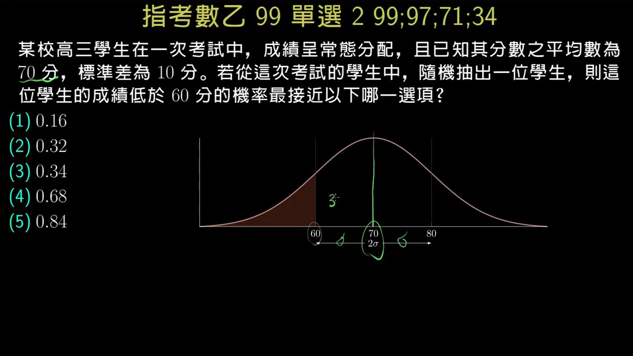
The video points out that the normal distribution is a bell-shaped curve; if comparing two normal curves, look at the mean for position and the standard deviation for shape. The mean determines the horizontal shift of the curve, and the standard deviation determines the width and height of the curve.
02
Mean Determines Left-Right Position
In this problem, School A's mean is 60 and School B's mean is 65. Because 65 > 60, School B's curve should be to the right of School A's. This is the first layer of condition when judging the graph.
03
Standard Deviation Determines Width and Concentration
Within the same normalized normal family and coordinate scale, larger standard deviation gives a wider curve with a lower peak; area1 alone does not determine the width-height relation of arbitrary densities.
04
Why Can't We Only Look at the Mean in This Problem
The speaker explicitly points out that all five options roughly satisfy "A on the left, B on the right," so the mean itself cannot distinguish the answer. What really separates the options is the shape difference caused by the standard deviation.
05
Continue eliminating by shape
Compare the widths of the thick and thin curves to eliminate diagrams that mismatch the normal parameters. Together with peak heights, A matches the two schools’ centers and scales.
06
Meaning of Area Under Normal Distribution Curve
In the graph of a probability density function, the total area enclosed by the curve and the horizontal axis represents the sum of probabilities of all possible outcomes, and its value is always equal to 1. This is the fundamental constraint condition for judging changes in the shape of distribution graphs.
∫−∞∞f(x)dx=1
07
Effect of Standard Deviation on Curve Shape
Within the same normalized normal family and coordinate scale, larger standard deviation gives a wider curve with a lower peak; area1 alone does not determine the width-height relation of arbitrary densities.
08
Effect of Mean on Curve Position
The mean is the symmetry center of a normal curve. With standard deviation fixed, increasing the mean translates the curve right and decreasing it translates left; the two schools have different standard deviations, so also compare width and peak height.
09
Problem Solving Practice: Identifying the Correct Distribution Graph
Facing the comparison between School A (SD=10) and School B (SD=5), first judge based on standard deviation that School A should be wider and shorter than School B, eliminating options with equal peak heights; second, judge based on the mean that School A (60) should be to the left of School B (65). Combining these two points allows locking onto the correct graph.
Detailed learning notes
Explore conditions, steps and evidence. Supplementary explanations are labeled separately from content shown in the video.
Symbols · 10
μ_A = 60
Clear evidence
Supplementary explanation
Evidence
Caption evidence
Observation
The problem text on screen states "The average score of students from School A is 60".
Audio
Observation
The narration compares centers by mean, then normal-curve width and peaks by standard deviation; the later area-1 explanation completes the selection of A.
Uncertainties
Editorial A/B labels denote the schools, distinct from diagram-option A/B.
Symbol
μ_A = 60
Meaning
The central position of the normal distribution of scores for School A, corresponding to the horizontal axis position of the curve's peak.
Domain
Mean parameter on the score scale
σ_A = 10
Clear evidence
Supplementary explanation
Evidence
Caption evidence
Observation
The problem text on screen states "standard deviation is 10" after the conditions for School A.
Audio
Observation
The narration compares centers by mean, then normal-curve width and peaks by standard deviation; the later area-1 explanation completes the selection of A.
Uncertainties
Editorial A/B labels denote the schools, distinct from diagram-option A/B.
Symbol
σ_A = 10
Meaning
The dispersion of the score distribution for School A; a larger standard deviation results in a wider, more spread-out curve.
Domain
Dispersion parameter on the score scale
μ_B = 65
Clear evidence
Supplementary explanation
Evidence
Caption evidence
Observation
The problem text on screen states "The average score of students from School B is 65".
Audio
Observation
The narration compares centers by mean, then normal-curve width and peaks by standard deviation; the later area-1 explanation completes the selection of A.
Uncertainties
Editorial A/B labels denote the schools, distinct from diagram-option A/B.
Symbol
μ_B = 65
Meaning
The center of School B’s normal curve:65 exceeds60, placing its center to the right of School A’s center, without separating their supports.
Domain
Mean parameter on the score scale
σ_B = 5
Clear evidence
Supplementary explanation
Evidence
Caption evidence
Observation
The problem text on screen states "standard deviation is 5" after the conditions for School B.
Audio
Observation
The narration compares centers by mean, then normal-curve width and peaks by standard deviation; the later area-1 explanation completes the selection of A.
Uncertainties
Editorial A/B labels denote the schools, distinct from diagram-option A/B.
Symbol
σ_B = 5
Meaning
The dispersion of the score distribution for School B; a smaller standard deviation results in a narrower, taller, and more concentrated curve.
Domain
Dispersion parameter on the score scale
A
Clear evidence
Supplementary explanation
Evidence
Caption evidence
Observation
The problem text states "If a thick line represents the score distribution curve of students from School A".
Audio
Observation
The narration compares centers by mean, then normal-curve width and peaks by standard deviation; the later area-1 explanation completes the selection of A.
Uncertainties
Editorial A/B labels denote the schools, distinct from diagram-option A/B.
Symbol
A
Meaning
The line style representing the normal distribution curve of School A in the option diagrams.
Domain
Legend line style
B
Clear evidence
Supplementary explanation
Evidence
Caption evidence
Observation
The problem text states "a thin line represents the score distribution curve of students from School B".
Audio
Observation
The narration compares centers by mean, then normal-curve width and peaks by standard deviation; the later area-1 explanation completes the selection of A.
Uncertainties
Editorial A/B labels denote the schools, distinct from diagram-option A/B.
Symbol
B
Meaning
The line style representing the normal distribution curve of School B in the option diagrams.
Domain
Legend line style
60
Clear evidence
Shown in the video
Evidence
Caption evidence
Observation
The problem text states 'The average score of students from School A is 60'.
Uncertainties
Compare the same normalized normal family on the same coordinate scale; area1 alone does not determine width and peak height for arbitrary densities.
Symbol
60
Meaning
Average test score of students from School A
Domain
Score
10
Clear evidence
Shown in the video
Evidence
Caption evidence
Observation
The problem text states 'The standard deviation is 10'.
Uncertainties
Compare the same normalized normal family on the same coordinate scale; area1 alone does not determine width and peak height for arbitrary densities.
Symbol
10
Meaning
Standard deviation of test scores for students from School A
Domain
Score
65
Clear evidence
Shown in the video
Evidence
Caption evidence
Observation
The problem text states 'The average score of students from School B is 65'.
Uncertainties
Compare the same normalized normal family on the same coordinate scale; area1 alone does not determine width and peak height for arbitrary densities.
Symbol
65
Meaning
Average test score of students from School B
Domain
Score
5
Clear evidence
Shown in the video
Evidence
Caption evidence
Observation
The problem text states 'The standard deviation is 5'.
Uncertainties
Compare the same normalized normal family on the same coordinate scale; area1 alone does not determine width and peak height for arbitrary densities.
Symbol
5
Meaning
Standard deviation of test scores for students from School B
Domain
Score
Knowledge points · 6
Position and shape of the normal distribution curve are determined by the mean and standard deviation
Clear evidence
Shown in the video
Evidence
Audio
Observation
The narration compares centers by mean, then normal-curve width and peaks by standard deviation; the later area-1 explanation completes the selection of A.
Caption evidence
Observation
The problem text explains that the score distributions of both schools are "very close to a normal distribution."
Definition
Explanation
The video describes the normal distribution as a bell-shaped curve and explicitly states that its "position" is determined by the mean and its "shape" is determined by the standard deviation. Therefore, when comparing two normal curves, one can first look at the mean to determine horizontal shift, and then look at the standard deviation to determine width and height.
Formula
Conditions
Distribution is close to a normal distribution
Comparison objects are two normal curves
The mean determines the horizontal position of the normal curve
Clear evidence
Supplementary explanation
Evidence
Audio
Observation
The narration compares centers by mean, then normal-curve width and peaks by standard deviation; the later area-1 explanation completes the selection of A.
Caption evidence
Observation
The problem states School A's mean score is 60 and School B's mean score is 65.
Method
Explanation
School B’s mean65 exceeds School A’s60, so its normal center, symmetry axis and peak location are to the right. This compares centers, not disjoint supports; the schools also have different standard deviations, so their curves are not simple rigid translations.
Formula
Conditions
Horizontal axis represents scores
Both schools' distributions are approximately normal
Prerequisites
Position and shape of the normal distribution curve are determined by the mean and standard deviation
The standard deviation determines the width and height of the normal curve
Clear evidence
Shown in the video
Evidence
Audio
Observation
The narration compares centers by mean, then normal-curve width and peaks by standard deviation; the later area-1 explanation completes the selection of A.
Caption evidence
Observation
The problem states School A's standard deviation is 10 and School B's standard deviation is 5.
Method
Explanation
The larger the standard deviation, the more dispersed the data, and the wider and flatter the curve; the smaller the standard deviation, the more concentrated the data, and the narrower and taller the curve. In this problem, School A's standard deviation of 10 is greater than School B's standard deviation of 5, so School A's curve should be wider and shorter than School B's.
Formula
Conditions
Both curves are normal distributions
Comparing dispersion under the same score scale
Prerequisites
Position and shape of the normal distribution curve are determined by the mean and standard deviation
Relationship between Area and Shape of Normal Distribution Curve
Clear evidence
Supplementary explanation
Evidence
Audio
Observation
The narration compares centers by mean, then normal-curve width and peaks by standard deviation; the later area-1 explanation completes the selection of A.
Uncertainties
Compare the same normalized normal family on the same coordinate scale; area1 alone does not determine width and peak height for arbitrary densities.
Definition
Explanation
The normalized normal densities in this question have total area1. Scaling the same normal family horizontally by its standard deviation inversely scales density height, with peak1/(σ√(2π)); arbitrary densities of area1 need not have this fixed width-height relation.
Formula
Conditions
Normalized normal location-scale family, positive standard deviation, same coordinate scale
Effect of Standard Deviation on Normal Distribution Curve Shape
Clear evidence
Shown in the video
Evidence
Audio
Observation
The narration compares centers by mean, then normal-curve width and peaks by standard deviation; the later area-1 explanation completes the selection of A.
Uncertainties
Compare the same normalized normal family on the same coordinate scale; area1 alone does not determine width and peak height for arbitrary densities.
Method
Explanation
The larger the standard deviation, the more dispersed the data, resulting in a wider and lower normal distribution curve; the smaller the standard deviation, the more concentrated the data, resulting in a narrower and higher normal distribution curve.
Formula
Conditions
Total area is always 1
Compare the same normal family, not arbitrary densities.
Prerequisites
Relationship between Area and Shape of Normal Distribution Curve
Effect of Mean on Normal Distribution Curve Position
Clear evidence
Supplementary explanation
Evidence
Audio
Observation
The narration compares centers by mean, then normal-curve width and peaks by standard deviation; the later area-1 explanation completes the selection of A.
Uncertainties
Compare the same normalized normal family on the same coordinate scale; area1 alone does not determine width and peak height for arbitrary densities.
Method
Explanation
The mean of a normal distribution sets its symmetry center. A pure horizontal translation holds only when the standard deviation is fixed and the mean alone changes; the schools have different standard deviations, so their complete curves are not simple translations.
Formula
Conditions
Single-parameter horizontal translation requires fixed standard deviation.
Claims and conditions · 2
School B's curve is located to the right of School A's curve
Clear evidence
Supplementary explanation
Evidence
Audio
Observation
The narration compares centers by mean, then normal-curve width and peaks by standard deviation; the later area-1 explanation completes the selection of A.
Caption evidence
Observation
School A's mean score is 60, School B's mean score is 65.
Proposition
Statement
School B’s mean65 exceeds School A’s60, so its normal center and peak location lie to the right of School A’s center. Both normal densities still have support on the entire real line; the curves are not disjoint.
Hypotheses
Score distributions of both schools are close to normal distributions
Horizontal axis is score and increases to the right
Quantifiers
Holds for the normal distribution curves of Schools A and B in this problem.
School A's curve is wider and more dispersed than School B's curve
Clear evidence
Shown in the video
Evidence
Audio
Observation
The narration compares centers by mean, then normal-curve width and peaks by standard deviation; the later area-1 explanation completes the selection of A.
Caption evidence
Observation
School A's standard deviation is 10, School B's standard deviation is 5.
Proposition
Statement
Because School A's standard deviation of 10 is greater than School B's standard deviation of 5, School A's normal curve should be wider, flatter, and more dispersed than School B's normal curve.
Hypotheses
Score distributions of both schools are close to normal distributions
Comparing curve shapes under the same coordinate scale
Quantifiers
Holds for the normal distribution curves of Schools A and B in this problem.
Derivations and proofs · 2
Using mean and standard deviation to eliminate options and determine the answer
Clear evidence
Supplementary explanation
Evidence
Audio
Observation
The narration compares centers by mean, then normal-curve width and peaks by standard deviation; the later area-1 explanation completes the selection of A.
Diagram
Observation
The screen displays five normal curve options (A) to (E), and the speaker makes circle and cross marks on the options.
Uncertainties
The video does not read out the final judgment sentence for each option verbatim; it relies on screen markings and semantic inference.
The first-segment model misread D. Native55 shows C crossed out;91 shows A circled. A is the later complete-source answer, not a completed selection at53–61seconds.
Visual argument
Steps
Expression
Explanation
First read the problem setup: School A mean 60, standard deviation 10; School B mean 65, standard deviation 5; thick line represents School A, thin line represents School B.
Justification
From the problem text and the speaker's oral description.
Shown in the video
Expression
Explanation
Compare positions by mean: 65 > 60, so School B's curve should be to the right of School A's.
Justification
The position of the normal curve is determined by the mean.
Shown in the video
Expression
Explanation
Observe the five options; the speaker points out that they all roughly satisfy "School A is more to the left, School B is more to the right," so relying solely on the mean cannot distinguish the options.
Justification
From the speaker's description of the common position of the five graphs.
Shown in the video
Expression
Explanation
Switch to comparing shapes by standard deviation: School A's standard deviation of 10 is larger, so School A's curve should be wider and more dispersed; School B's standard deviation of 5 is smaller, so School B's curve should be narrower and more concentrated.
Justification
The shape of the normal curve is determined by the standard deviation.
Shown in the video
Expression
Explanation
Check the relative width and height of the thick and thin lines in the graphs item by item, eliminating options that do not fit "thick line is wider, thin line is narrower and shifted right."
Justification
Translate problem parameters into graphical features and compare.
Shown in the video
Expression
Explanation
This segment begins eliminating mismatched shapes; the full source later confirms A, rather than showing a completed D selection here.
Justification
Actual55 and91 native frames distinguish the current stage from the complete-source conclusion.
Supplementary explanation
Conclusion
This stage establishes location and spread checks; the later complete-source answer is A.
Problem Solving Derivation Process
Clear evidence
Shown in the video
Evidence
Audio
Observation
The narration compares centers by mean, then normal-curve width and peaks by standard deviation; the later area-1 explanation completes the selection of A.
Uncertainties
Compare the same normalized normal family on the same coordinate scale; area1 alone does not determine width and peak height for arbitrary densities.
Intuitive argument
Steps
Expression
Explanation
Observe options A and B; in both, the thick line (School A) is wider, and the thin line (School B) is narrower.
Justification
Visual observation
Shown in the video
Expression
Explanation
According to the problem, School A's standard deviation (10) is greater than School B's standard deviation (5), so School A's curve should be wider and lower than School B's.
Justification
Standard deviation affects curve width and height
Derived from the video
Expression
Explanation
In option B, the peak heights of the two curves are identical, which does not match the height difference caused by different standard deviations.
Justification
Peak height in the same normalized normal family is inversely proportional to positive standard deviation; the distinct10 and5 scales cannot give equal peaks.
Supplementary explanation
Expression
Explanation
In option A, the thick line (School A) is wider and shorter, while the thin line (School B) is narrower and taller, consistent with the properties of standard deviation.
Justification
Intuitive comparison
Shown in the video
Conclusion
The correct answer is (A).
Worked examples · 2
CSAT Math 101 Multiple Choice 4: Interpreting Normal Distribution Graphs of Two Schools' Scores
Clear evidence
Supplementary explanation
Evidence
Caption evidence
Observation
The screen fully presents the problem: Students from Schools A and B took a math ability test, and their scores are both close to a normal distribution; School A mean 60, standard deviation 10; School B mean 65, standard deviation 5; thick line represents School A, thin line represents School B, asking which distribution graph is more correct.
Audio
Observation
The narration compares centers by mean, then normal-curve width and peaks by standard deviation; the later area-1 explanation completes the selection of A.
Uncertainties
The first-segment model misread D. Native55 shows C crossed out;91 shows A circled. A is the later complete-source answer, not a completed selection at53–61seconds.
Problem
Students from Schools A and B, who have the same number of students, took a math ability test. The distribution of test scores for students from both schools is very close to a normal distribution. Among them, the average score of students from School A is 60, with a standard deviation of 10; the average score of students from School B is 65, with a standard deviation of 5. If a thick line represents the score distribution curve of students from School A, and a thin line represents the score distribution curve of students from School B, then which of the following distribution graphs is more correct?
Given
School A mean score = 60
School A standard deviation = 10
School B mean score = 65
School B standard deviation = 5
Thick line represents School A
Thin line represents School B
Score distributions of both schools are close to normal distributions
Goal
Select the distribution graph that best fits the problem setup from the five normal curve graphs (A) to (E).
Steps
Expression
Explanation
First judge the horizontal position: Because School B's mean of 65 is greater than School A's mean of 60, School B's curve should be to the right of School A's.
Justification
The position of the normal distribution curve is determined by the mean.
Shown in the video
Expression
Explanation
Then judge the shape: Because School A's standard deviation of 10 is greater than School B's standard deviation of 5, School A's curve should be wider, flatter, and more dispersed than School B's.
Justification
The shape of the normal distribution curve is determined by the standard deviation.
Shown in the video
Expression
Explanation
Combine with line style conditions: The wider curve on the left should be the thick line (School A), and the narrower and taller curve on the right should be the thin line (School B).
Justification
The problem specifies that the thick line represents School A and the thin line represents School B.
Shown in the video
Expression
Explanation
Combine the mean and standard-deviation conditions to compare the options; the full source later confirms A’s broad low thick curve left and narrow high thin curve right.
Justification
The complete answer follows the actual later A marking; the first segment does not mark a final answer.
Supplementary explanation
Answer
Full-source answer A; current0–61seconds establishes the comparison conditions.
Verification
Can be checked with two conditions: ① Is the peak of the thin line to the right of the thick line? ② Is the thick line wider and shorter than the thin line? Option (A) satisfies both.
CSAT Math 101 Multiple Choice 4: Comparing Grade Normal Distribution Graphs
Clear evidence
Shown in the video
Evidence
Caption evidence
Observation
The full problem statement is displayed at the top of the screen.
Uncertainties
Compare the same normalized normal family on the same coordinate scale; area1 alone does not determine width and peak height for arbitrary densities.
Problem
Schools A and B have an equal number of students taking a mathematics ability test. The distribution of test scores for students from both schools is close to a normal distribution. The average score for students from School A is 60, with a standard deviation of 10; the average score for students from School B is 65, with a standard deviation of 5. If the thick line represents the score distribution curve for School A and the thin line represents the score distribution curve for School B, which of the following distribution graphs is most correct?
Given
School A average score = 60
School A standard deviation = 10
School B average score = 65
School B standard deviation = 5
Thick line represents School A, thin line represents School B
Goal
Select the correct distribution graph option (A)-(E)
Steps
Expression
Explanation
Compare standard deviations: School A (10) > School B (5), so School A's curve should be wider and shorter than School B's.
Justification
Within the same normal family, larger standard deviation increases horizontal scale and lowers the peak.
Derived from the video
Expression
Explanation
Compare means: School A (60) < School B (65), so the center of School A's curve should be to the left of School B's.
Justification
Mean determines the position of the curve's axis of symmetry
Derived from the video
Expression
Explanation
Examine options: (C), (D), and (E) have been crossed out and eliminated. Between (A) and (B), (B) has two curves of equal height, which does not fit the standard deviation difference; (A) has a shorter and wider thick line, and a taller and narrower thin line, with the thick line on the left and the thin line on the right.
Justification
Graph feature matching
Shown in the video
Answer
(A)
Verification
Option A satisfies both the width/height difference caused by standard deviation and the left/right position difference caused by the mean.
Visual events · 8
Layout of the full page problem and five option graphs
Clear evidence
Shown in the video
Evidence
Diagram
Observation
The screen is a single-page problem with white text on a black background. At the top is a yellow title "CSAT Math 101 Multiple Choice 4 86;77;45;15", the middle section is the problem text, and the bottom has five normal curve graphs (A) to (E) arranged horizontally. In the lower left corner, there is a green option list (1)(A) to (5)(E).
Objects
Title bar
Problem text
Five normal curve graphs (A) to (E)
Option list in lower left corner
Changes
No scene switching; the entire segment maintains the same problem page.
Invariants
Problem text and five option graphs remain visible throughout.
Interpretation
This is a static problem page where the solution is completed through oral explanation and subsequent marking, rather than explaining concepts through animation changes.
Marking key terms in the problem stem with green underlines
Clear evidence
Shown in the video
Evidence
Animation
Observation
Green underlines appear sequentially below keywords such as "normal distribution", "average score is 60", and "average score is 65".
Audio
Observation
The narration compares centers by mean, then normal-curve width and peaks by standard deviation; the later area-1 explanation completes the selection of A.
Objects
Problem stem text
Green underlines
Changes
First marks "normal distribution", then marks School A's mean of 60 and School B's mean of 65.
Invariants
Problem layout remains unchanged, only emphasis marks are added.
Interpretation
Visually separates the core parameters needed for solving: first confirm the distribution type, then confirm the means of the two schools.
Circling the standard deviations of both schools as the second layer of criteria
Clear evidence
Shown in the video
Evidence
Animation
Observation
Green ellipses circle "standard deviation is 10" and "standard deviation is 5".
Audio
Observation
The narration compares centers by mean, then normal-curve width and peaks by standard deviation; the later area-1 explanation completes the selection of A.
Objects
Standard deviation text in the problem stem
Green ellipse circling mark
Changes
After marking the means, further shifts attention to the standard deviation conditions.
Invariants
The five option graphs remain unmodified.
Interpretation
This step shifts the focus of solving from "position" to "shape," corresponding to the real distinguishing point of this problem.
Begin eliminating diagrams by spread
Clear evidence
Supplementary explanation
Evidence
Animation
Observation
Actual native55: C is crossed out and A not yet circled. Later native91: A is circled, with B/C/D/E crossed out.
Audio
Observation
The narration compares centers by mean, then normal-curve width and peaks by standard deviation; the later area-1 explanation completes the selection of A.
Uncertainties
Some intermediate marks appear for a short moment; the exact seconds of pen strokes can only be approximated.
The first-segment model misread D. Native55 shows C crossed out;91 shows A circled. A is the later complete-source answer, not a completed selection at53–61seconds.
Objects
Five option graphs (A) to (E)
Green crosses
Green circle marks
Option list in lower left corner
Changes
C has a green cross at this stage; A is circled later.
Invariants
Problem stem text remains unchanged.
Interpretation
Native55 shows C crossed out,91 shows A circled; the first-segment mark is elimination, not selection of D.
Marking Incorrect Option B
Clear evidence
Shown in the video
Evidence
Animation
Observation
Green pen marks draw an 'X' over option (B).
Uncertainties
Compare the same normalized normal family on the same coordinate scale; area1 alone does not determine width and peak height for arbitrary densities.
Objects
Graph for option (B)
Changes
Green 'X' appears
Invariants
Other options remain unchanged
Interpretation
The speaker determines that option B does not conform to the relationship between area and height in a normal distribution and eliminates it.
Marking Correct Option A
Clear evidence
Shown in the video
Evidence
Animation
Observation
Green pen marks circle the letter for option (A).
Uncertainties
Compare the same normalized normal family on the same coordinate scale; area1 alone does not determine width and peak height for arbitrary densities.
Objects
Letter for option (A)
Changes
Green circle appears
Invariants
Other options remain unchanged
Interpretation
The speaker confirms A as the correct answer.
Demonstrating Area and Height Relationship
Clear evidence
Supplementary explanation
Evidence
Animation
Observation
Green pen marks shade the area under the thick line in option (A) and draw vertical lines above the thin line.
Uncertainties
Compare the same normalized normal family on the same coordinate scale; area1 alone does not determine width and peak height for arbitrary densities.
Objects
Curves in option (A)
Changes
Green shaded area appears under the thick line
Green vertical auxiliary lines appear next to the thin line
Invariants
Curve shapes themselves remain unchanged
Interpretation
The source gives a area-1 intuition; the precise inverse width-height relation concerns scale changes within the same normalized normal family, not arbitrary densities.
Boxing Final Answer
Clear evidence
Shown in the video
Evidence
Animation
Observation
Green pen marks draw a box around the answer area (1)(A) in the bottom left corner.
Uncertainties
Compare the same normalized normal family on the same coordinate scale; area1 alone does not determine width and peak height for arbitrary densities.
Objects
Answer area (1)(A)
Changes
Green box appears
Invariants
None
Interpretation
Emphasizes that the final selected answer is (1)(A).
Misconceptions · 3
Looking only at the mean is not enough to distinguish the options in this problem
Clear evidence
Shown in the video
Evidence
Audio
Observation
The narration compares centers by mean, then normal-curve width and peaks by standard deviation; the later area-1 explanation completes the selection of A.
Misconception
Thinking that just judging "B is to the right of A" is enough to select the correct graph.
Clarification
In the video, all five options roughly satisfy A on the left and B on the right, so one must further use the standard deviation to compare curve widths to filter further.
Do not mistake a larger standard deviation for a taller and narrower curve
Clear evidence
Derived from the video
Evidence
Audio
Observation
The narration compares centers by mean, then normal-curve width and peaks by standard deviation; the later area-1 explanation completes the selection of A.
Misconception
It is easy to intuitively associate "larger value" with "taller curve," mistakenly thinking that a curve with a larger standard deviation is sharper and taller.
Clarification
According to the video, a larger standard deviation means the data is more dispersed, and the curve should be wider and flatter; a smaller standard deviation means it is more concentrated, narrower, and taller. This item is an error-prone reminder organized by the analyst based on reasoning from the video.
Misconception that Standard Deviation Does Not Affect Curve Height
Clear evidence
Supplementary explanation
Evidence
Audio
Observation
The narration compares centers by mean, then normal-curve width and peaks by standard deviation; the later area-1 explanation completes the selection of A.
Uncertainties
Compare the same normalized normal family on the same coordinate scale; area1 alone does not determine width and peak height for arbitrary densities.
Misconception
Believing that as long as the means are different or only the widths are different, the highest point (peak) of the curve can remain the same height.
Clarification
For normalized normal densities on the same axes, the peak is1/(σ√(2π)); larger positive standard deviation gives a lower peak. Area1 alone does not imply this for arbitrary densities.
Concept relations · 6
The mean determines the horizontal position of the normal curve → School B's curve is located to the right of School A's curve
Clear evidence
Supplementary explanation
Evidence
Audio
Observation
The narration compares centers by mean, then normal-curve width and peaks by standard deviation; the later area-1 explanation completes the selection of A.
Application
Explanation
Comparing means locates the relative normal centers: School B’s center is to the right of School A’s center, without separating the curves’ supports.
The standard deviation determines the width and height of the normal curve → School A's curve is wider and more dispersed than School B's curve
Clear evidence
Shown in the video
Evidence
Audio
Observation
The narration compares centers by mean, then normal-curve width and peaks by standard deviation; the later area-1 explanation completes the selection of A.
Application
Explanation
The method "standard deviation determines width and height" is directly applied to this problem, yielding the conclusion that School A's curve is wider and more dispersed than School B's.
Position and shape of the normal distribution curve are determined by the mean and standard deviation → The mean determines the horizontal position of the normal curve
Clear evidence
Shown in the video
Evidence
Audio
Observation
The narration compares centers by mean, then normal-curve width and peaks by standard deviation; the later area-1 explanation completes the selection of A.
Contains
Explanation
The general property "normal curve is determined by mean and standard deviation" contains two sub-criteria, one of which is that the mean controls position.
Position and shape of the normal distribution curve are determined by the mean and standard deviation → The standard deviation determines the width and height of the normal curve
Clear evidence
Shown in the video
Evidence
Audio
Observation
The narration compares centers by mean, then normal-curve width and peaks by standard deviation; the later area-1 explanation completes the selection of A.
Contains
Explanation
The general property also contains another sub-criterion, namely that the standard deviation controls shape and dispersion.
Effect of Standard Deviation on Normal Distribution Curve Shape → Relationship between Area and Shape of Normal Distribution Curve
Clear evidence
Shown in the video
Evidence
Audio
Observation
The narration compares centers by mean, then normal-curve width and peaks by standard deviation; the later area-1 explanation completes the selection of A.
Uncertainties
Compare the same normalized normal family on the same coordinate scale; area1 alone does not determine width and peak height for arbitrary densities.
Application
Explanation
Applies the properties of standard deviation to understand changes in the shape of the normal distribution curve.
Effect of Mean on Normal Distribution Curve Position → CSAT Math 101 Multiple Choice 4: Comparing Grade Normal Distribution Graphs
Clear evidence
Shown in the video
Evidence
Audio
Observation
The narration compares centers by mean, then normal-curve width and peaks by standard deviation; the later area-1 explanation completes the selection of A.
Uncertainties
Compare the same normalized normal family on the same coordinate scale; area1 alone does not determine width and peak height for arbitrary densities.
Application
Explanation
Uses the property that the mean determines curve position to solve the problem.
Find an answer · 7
Why is School B's normal curve drawn to the right of School A's?
Clear evidence
Shown in the video
Evidence
Audio
Observation
The narration compares centers by mean, then normal-curve width and peaks by standard deviation; the later area-1 explanation completes the selection of A.
Knowledge points
The mean determines the horizontal position of the normal curve
School B's curve is located to the right of School A's curve
Why can't this problem rely only on the mean to select the graph, but also needs to look at the standard deviation?
Clear evidence
Shown in the video
Evidence
Audio
Observation
The narration compares centers by mean, then normal-curve width and peaks by standard deviation; the later area-1 explanation completes the selection of A.
Knowledge points
The standard deviation determines the width and height of the normal curve
Looking only at the mean is not enough to distinguish the options in this problem
When the standard deviation is larger, does the normal curve become wider or taller?
Clear evidence
Shown in the video
Evidence
Audio
Observation
The narration compares centers by mean, then normal-curve width and peaks by standard deviation; the later area-1 explanation completes the selection of A.
Knowledge points
The standard deviation determines the width and height of the normal curve
School A's curve is wider and more dispersed than School B's curve
Why was (A) selected in the end for this problem?
Clear evidence
Supplementary explanation
Evidence
Diagram
Observation
The screen finally circles (A), and (1)(A) in the lower left corner is also circled.
Uncertainties
The first-segment model misread D. Native55 shows C crossed out;91 shows A circled. A is the later complete-source answer, not a completed selection at53–61seconds.
Knowledge points
Using mean and standard deviation to eliminate options and determine the answer
CSAT Math 101 Multiple Choice 4: Interpreting Normal Distribution Graphs of Two Schools' Scores
Why can't the peak heights be the same when comparing two normal distributions with different standard deviations?
Clear evidence
Shown in the video
Evidence
Audio
Observation
The narration compares centers by mean, then normal-curve width and peaks by standard deviation; the later area-1 explanation completes the selection of A.
Uncertainties
Compare the same normalized normal family on the same coordinate scale; area1 alone does not determine width and peak height for arbitrary densities.
Knowledge points
Relationship between Area and Shape of Normal Distribution Curve
Misconception that Standard Deviation Does Not Affect Curve Height
How does the magnitude of the standard deviation affect the width and height of the normal distribution curve?
Clear evidence
Shown in the video
Evidence
Audio
Observation
The narration compares centers by mean, then normal-curve width and peaks by standard deviation; the later area-1 explanation completes the selection of A.
Uncertainties
Compare the same normalized normal family on the same coordinate scale; area1 alone does not determine width and peak height for arbitrary densities.
Knowledge points
Effect of Standard Deviation on Normal Distribution Curve Shape
What does the mean represent in a normal distribution graph?
Clear evidence
Shown in the video
Evidence
Audio
Observation
The narration compares centers by mean, then normal-curve width and peaks by standard deviation; the later area-1 explanation completes the selection of A.
Uncertainties
Compare the same normalized normal family on the same coordinate scale; area1 alone does not determine width and peak height for arbitrary densities.
Knowledge points
Effect of Mean on Normal Distribution Curve Position
Coverage and review notes
Covered · Starts by reading the problem and pointing out that the score distributions of both schools are close to normal distributions.
Covered · The speaker explains that the normal distribution is a bell-shaped curve, and its position and shape are affected by the mean and standard deviation.
Covered · Extracts the means of Schools A and B and the correspondence of thick/thin lines, deducing that B is to the right of A.
Covered · The speaker points out that all five graphs roughly satisfy A on the left and B on the right, so one needs to switch to using standard deviation for discrimination.
Covered · Extracts the standard deviations of both schools, explaining that a larger standard deviation means the curve is fatter and more dispersed.
Covered · At53–61seconds the spread comparison begins eliminating options; the later full-source segment completes the choice of A.
Covered · Reading the problem and beginning to compare graphical features of options A and B.
Covered · Use the inverse scaling of area-normalized curves within the same normal family to explain the intuition, eliminate B and confirm A; area1 alone is not a width-height theorem for arbitrary densities.
Covered · Summarizing the rules that standard deviation affects shape and mean affects position, and boxing the final answer.
A score-distribution question separates the location and shape of normal curves. School A has mean60 and standard deviation10; School B has mean65 and standard deviation5. The thick line represents School A, and the thin line School B. School A must have a leftward center and a wider, lower peak; School B a rightward center and a narrower, higher peak. The complete source selects diagram A. The question describes real scores as close to normal, so the comparison uses a normal model. The area-1 intuition applies to the same normalized normal family on the same coordinate scale, not to arbitrary densities merely sharing area 1.
The video points out that the normal distribution is a bell-shaped curve; if comparing two normal curves, look at the mean for position and the standard deviation for shape. The mean determines the horizontal shift of the curve, and the standard deviation determines the width and height of the curve.
 math
math