Reviewed learning material · Video analysis · EnglishRead the full overview
This lecture segment introduces the concept of numerical stability as a property of a function's computer implementation, distinguishing it from the inherent conditioning of the mathematical function itself. Using a blackboard diagram, the speaker illustrates how an exact function f maps an input x to an output f(x), while an implementation fˇ maps the same input to a potentially different output fˇ(x). The speaker emphasizes that even a highly stable implementation cannot overcome the large output errors caused by an ill-conditioned function, where small input changes (like measurement errors) lead to disproportionately large output variations.
This video segment introduces the fundamental concepts of numerical stability and backward error analysis in computational mathematics. Using a blackboard mapping diagram, the instructor explains that a numerically stable algorithm produces a computed result that is exactly equal to the true mathematical function evaluated at a slightly perturbed input. He then defines backward error analysis as the method used to verify this property by working backward from the computed output to find the corresponding approximate input, ensuring that computational errors like floating-point rounding do not cause significant deviations from the function's true behavior.
Use the learning inspector for key ideas and moments, or open the reading tabs for the complete notes.
Generated from the video's visuals and explanation; not verbatim speech.
The lecture begins by introducing the core topic: numerical stability. The speaker defines this as a specific property of how a mathematical function is implemented on a computer, rather than a property of the abstract function itself.
To illustrate this, a blackboard diagram is drawn showing an exact function f mapping an input x from a domain D to an output f(x) in a range R. This represents ideal, exact arithmetic.
The speaker then contrasts this with reality: computer implementations suffer from round-off errors and potential bugs. A second mapping is added to the diagram, showing an implemented function fˇ taking the same input x but producing a different output fˇ(x).
The central question of numerical stability is posed: when is an implementation considered 'good'? Visually, the outputs f(x) and fˇ(x) are drawn far apart to represent a poor implementation with high error.
However, the speaker introduces a crucial distinction: conditioning. Even with a highly stable implementation (where fˇ(x) is very close to f(x)), an ill-conditioned function will amplify tiny input errors—such as those from physical measurements—into massive output discrepancies. Thus, stability and conditioning are fundamentally different properties.
The segment concludes by setting up the formal quantification of stability. The speaker introduces a perturbed input xˇ near x on the diagram, preparing to define a stable implementation as one where the output fˇ(xˇ) remains close to the true function's behavior, despite the input shift.
In numerical computing, we often deal with functions mapping a domain D to a codomain R, denoted as f: D -> R. When we implement this function on a computer, we introduce small perturbations. The original input x might become a slightly altered input x~ due to measurement errors, floating-point storage limitations, or rounding errors during the evaluation of the mathematical expression itself.
Despite these inevitable small errors, we want our algorithm to behave predictably. An algorithm is defined as numerically stable if the computed output, let's call it f~(x), is exactly equal to the true function f evaluated at some nearby, perturbed input x~. In other words, f~(x)=f(x~). This means the algorithm isn't amplifying tiny input errors into massive, unpredictable output errors; it's simply giving us the exact answer for a slightly different question.
To rigorously check if an algorithm meets this standard of stability, mathematicians use a technique called backward error analysis. Instead of tracking how an initial error in x propagates forward through the computation to ruin the final result, backward error analysis works in reverse. It takes the final computed result f~(x) and asks: 'For what exact input x~ would the true function f naturally produce this specific output?' If the calculated x~ is very close to our original intended input x, we have successfully proven that the algorithm is numerically stable. This framework is essential for analyzing complex operations in fields like linear algebra.
Knowledge cards
01
Definition of Numerical Stability
Numerical stability is a property of a function's computer implementation. It measures how closely the implemented algorithm approximates the exact mathematical function, accounting for inevitable computational errors like floating-point round-off.
02
Exact Function vs. Implemented Function
An exact function f maps an input x to a precise output f(x) under ideal arithmetic. In contrast, an implemented function fˇ maps the same input x to an approximate output fˇ(x) due to computational limitations and potential software bugs.
f(x)=fˇ(x)
03
Conditioning of a Mathematical Problem
Conditioning describes the inherent sensitivity of a mathematical function to small changes in its input. An ill-conditioned function will produce a disproportionately large change in its output for even a microscopic perturbation in the input, regardless of how perfectly the algorithm is coded.
04
Stability vs. Conditioning
It is a common misconception that a highly stable algorithm can solve any problem accurately. However, if the underlying mathematical problem is ill-conditioned, small input errors (e.g., from measurement) will inevitably lead to large output errors, making the problem inherently difficult to solve accurately.
05
Numerically Stable Algorithm
An algorithm is numerically stable if its computed output f~(x) is exactly equal to the true mathematical function f evaluated at a slightly perturbed input x~. This ensures that small computational errors (like floating-point rounding) do not cause the result to deviate wildly from the function's true behavior for nearby inputs.
f~(x)=f(x~)
06
Backward Error Analysis
A method used to prove numerical stability. Rather than tracking how input errors propagate forward to affect the output, it works backward: given a computed output, it determines what exact input would produce that output via the true function. If this 'backward' input is close to the original intended input, the algorithm is stable.
Detailed learning notes
Explore conditions, steps and evidence. Supplementary explanations are labeled separately from content shown in the video.
Symbols · 15
f
Clear evidence
Shown in the video
Evidence
Formula
Observation
Written on the blackboard as 'f: D -> R'.
Audio
Observation
The speaker refers to it as 'a function that maps elements of a domain to elements of a range'.
Symbol
f
Meaning
An exact mathematical function mapping from a domain to a range.
Domain
D
D
Clear evidence
Shown in the video
Evidence
Formula
Observation
Written on the blackboard as 'D' inside an oval shape.
Audio
Observation
The speaker refers to it as 'a domain'.
Symbol
D
Meaning
The domain of the function f.
Domain
Not stated in the source.
R
Clear evidence
Shown in the video
Evidence
Formula
Observation
Written on the blackboard as 'R' inside an oval shape.
Audio
Observation
The speaker refers to it as 'a range'.
Symbol
R
Meaning
The range of the function f.
Domain
Not stated in the source.
x
Clear evidence
Shown in the video
Evidence
Formula
Observation
Written on the blackboard inside the domain oval D.
Audio
Observation
The speaker says 'in goes some value x'.
Symbol
x
Meaning
An input value belonging to the domain D.
Domain
D
f(x)
Clear evidence
Shown in the video
Evidence
Formula
Observation
Written on the blackboard inside the range oval R.
Audio
Observation
The speaker says 'this gets mapped to some other value... f(x)'.
Symbol
f(x)
Meaning
The exact output value of the function f for the input x.
Domain
R
fˇ
Clear evidence
Shown in the video
Evidence
Formula
Observation
Written on the blackboard above a second arrow from x to R.
Audio
Observation
The speaker says 'an alternative function f check'.
Symbol
fˇ
Meaning
The implemented function on a computer, which may differ from the exact function f due to errors or bugs.
Domain
D
fˇ(x)
Clear evidence
Shown in the video
Evidence
Formula
Observation
Written on the blackboard inside the range oval R, below f(x).
Audio
Observation
The speaker says 'will map it to some other value using your implementation'.
Symbol
fˇ(x)
Meaning
The output value produced by the implemented function fˇ for the input x.
Domain
R
xˇ
Clear evidence
Shown in the video
Evidence
Formula
Observation
Written on the blackboard inside the domain oval D, near x.
Audio
Observation
The speaker says 'for a value close to x, let's call it x check'.
Symbol
xˇ
Meaning
A value in the domain D that is close to the original input x.
Domain
D
f
Clear evidence
Shown in the video
Evidence
Formula
Observation
Written on the blackboard as f: D -> R.
Symbol
f
Meaning
The original mathematical function being analyzed.
Domain
D
D
Clear evidence
Shown in the video
Evidence
Formula
Observation
Written on the blackboard as part of f: D -> R, and drawn as a large oval on the left.
Symbol
D
Meaning
The domain of the function f.
Domain
Set of all possible inputs
R
Clear evidence
Shown in the video
Evidence
Formula
Observation
Written on the blackboard as part of f: D -> R, and drawn as a large oval on the right.
Symbol
R
Meaning
The codomain (or range) of the function f.
Domain
Set of real numbers
x
Clear evidence
Shown in the video
Evidence
Formula
Observation
Written inside the domain oval D on the blackboard.
Symbol
x
Meaning
An exact input value to the function f.
Domain
D
Knowledge points · 4
Numerical Stability
Clear evidence
Shown in the video
Evidence
Audio
Observation
The speaker introduces the topic: 'We now arrive at the very important topic of numerical stability.'
Audio
Observation
The speaker defines it: 'Numerical stability is a property of the implementation of a function.'
Definition
Explanation
Numerical stability is a property of how well a computer implementation of a mathematical function approximates the exact function. It is distinct from the conditioning of the function itself, which measures how sensitive the exact function is to small changes in its input.
Formula
Conditions
Applies to the implementation of a function on a computer.
Conditioning of a Function
Clear evidence
Shown in the video
Evidence
Audio
Observation
The speaker explains: 'if the function is very sensitive to small changes, if its conditioning is bad, if it's ill-conditioned, then a small change in the input may result in a large change in the output regardless of how good your implementation is'.
Definition
Explanation
Conditioning refers to the inherent sensitivity of a mathematical function to small changes in its input. An ill-conditioned function will produce a large change in its output even for a tiny change in its input, making it difficult to compute accurately regardless of the implementation's quality.
Formula
Conditions
Inherent property of the mathematical function itself, independent of implementation.
Prerequisites
Numerical Stability
Definition of Numerically Stable Algorithm
Clear evidence
Shown in the video
Evidence
Audio
Observation
The speaker defines a numerically stable algorithm as one where the computed result can be attributed to an input close to the original input.
Definition
Explanation
An algorithm is considered numerically stable if the result it computes is exactly equal to the true mathematical function evaluated at some slightly perturbed input. This means that any errors introduced during computation (like floating-point rounding) do not cause the output to deviate wildly from the true behavior of the function for nearby inputs.
Formula
f~(x)=f(x~)
Conditions
The perturbation x~−x must be small.
Concept of Backward Error Analysis
Clear evidence
Shown in the video
Evidence
Audio
Observation
The speaker states that analyzing whether an algorithm has the property of numerical stability by attributing computed values to close inputs is called backward error analysis.
Method
Explanation
Backward error analysis is a technique used to evaluate the numerical stability of an algorithm. Instead of looking forward at how input errors propagate to output errors, it works backward: it asks what exact input would produce the computed output if passed through the true mathematical function. If this 'backward' input is very close to the original intended input, the algorithm is deemed stable.
Conditions
Used to prove or analyze the numerical stability of algorithms.
Prerequisites
Definition of Numerically Stable Algorithm
Visual events · 2
Function Mapping Diagram
Clear evidence
Shown in the video
Evidence
Diagram
Observation
Blackboard drawing showing two ovals labeled D and R, with arrows mapping x to f(x) via f, and x to fˇ(x) via fˇ.
Objects
Oval D (Domain)
Oval R (Range)
Point x
Point f(x)
Point fˇ(x)
Arrow f
Arrow fˇ
Point xˇ
Changes
The speaker draws the initial diagram for the exact function f.
The speaker adds a second arrow and output point for the implemented function fˇ.
The speaker adds a new point xˇ near x in the domain.
Invariants
The domain D and range R remain fixed.
The exact function f and its output f(x) remain fixed.
Interpretation
The diagram visually contrasts the exact mathematical function f with its computer implementation fˇ. The distance between the outputs f(x) and fˇ(x) represents the error introduced by the implementation. The addition of xˇ sets up the discussion on how input perturbations affect the output, relating to the function's conditioning.
Mapping Diagram for Function and Perturbed Inputs
Clear evidence
Shown in the video
Evidence
Diagram
Observation
A mapping diagram showing two ovals labeled D and R. Inside D are points x and x~. Inside R are points f(x) and f~(x). Arrows show f mapping x to f(x), and another arrow shows the computed result f~(x) corresponding to f(x~).
Objects
Domain set D
Codomain set R
Exact input x
Perturbed input x~
Exact output f(x)
Computed output f~(x)
Mapping arrows
Changes
The speaker points to different parts of the diagram while explaining the concepts of exact inputs, perturbed inputs, and computed outputs.
Invariants
The overall structure of the mapping diagram remains constant throughout the clip.
Interpretation
The diagram visually represents the core concept of backward error analysis: a computed output f~(x) is viewed as the exact output f(x~) of the true function for some slightly modified input x~.
Misconceptions · 1
Confusing Implementation Error with Conditioning
Clear evidence
Shown in the video
Evidence
Audio
Observation
The speaker clarifies: '...regardless of how good your implementation is, because you know you're going to incur error along the way. There might even have been error in the input when you measured it.'
Misconception
Believing that a highly accurate computer implementation can perfectly compute the output of an ill-conditioned function without significant error.
Clarification
Even with a perfect implementation, an ill-conditioned function will amplify any small errors present in the input data (e.g., from measurement), leading to large errors in the output. Numerical stability addresses the implementation's error, while conditioning addresses the problem's inherent sensitivity.
Concept relations · 2
Numerical Stability → Conditioning of a Function
Clear evidence
Shown in the video
Evidence
Audio
Observation
The speaker contrasts the two concepts: '...if its conditioning is bad... then a small change in the input may result in a large change in the output regardless of how good your implementation is'.
Contrast
Explanation
Numerical stability is a property of the algorithm's implementation, whereas conditioning is an inherent property of the mathematical problem itself. A stable algorithm minimizes implementation error, but it cannot overcome the large output variations caused by an ill-conditioned problem.
Concept of Backward Error Analysis → Definition of Numerically Stable Algorithm
Clear evidence
Shown in the video
Evidence
Audio
Observation
The speaker links the definition of numerical stability directly to the method of backward error analysis.
Application
Explanation
Backward error analysis is the specific methodological approach used to demonstrate and prove that an algorithm possesses the property of numerical stability.
Find an answer · 4
What is numerical stability?
Clear evidence
Shown in the video
Evidence
Audio
Observation
The speaker introduces the topic and defines it.
Knowledge points
Numerical Stability
How does numerical stability differ from the conditioning of a function?
Clear evidence
Shown in the video
Evidence
Audio
Observation
The speaker explains how ill-conditioning affects the output regardless of implementation quality.
Knowledge points
Numerical Stability
Conditioning of a Function
s0-cr-stability-cond
Confusing Implementation Error with Conditioning
What is the definition of a numerically stable algorithm?
Clear evidence
Shown in the video
Evidence
Audio
Observation
Speaker provides the definition of a numerically stable algorithm.
Knowledge points
Definition of Numerically Stable Algorithm
What is backward error analysis in numerical computing?
Clear evidence
Shown in the video
Evidence
Audio
Observation
Speaker introduces the term backward error analysis.
Knowledge points
Concept of Backward Error Analysis
Coverage and review notes
Covered · Introductory title sequence with music; no mathematical content.
Covered · Lecture segment introducing numerical stability, contrasting it with function conditioning, and illustrating the concepts with a blackboard diagram.
Covered · Introduction to the concept of small changes in inputs and evaluation leading to errors, setting up the definition of stability.
Covered · Explicit definition of a numerically stable algorithm.
Covered · Explanation of backward error analysis as the method to prove stability.
Covered · Outro screen with website URL, no mathematical content.
Reviewed English material v1: card "Conditioning of a Mathematical Problem" at 1:44 — Conditioning describes the inherent sensitivity of a mathematical function to small changes in its input. An ill-conditioned function will produce a disproportionately large change in its output for even a microscopic perturbation in the input, regardless of how perfectly the algorithm is coded.