Reviewed learning material · Video analysis · EnglishRead the full overview
This 150-second introductory clip explains linear regression visually and verbally. It first assigns the independent variable to the X-axis and the dependent variable to the Y-axis, then defines positive and negative relationships by whether the two variables move in the same or opposite directions. The narrator stresses that linear regression uses a straight line, plots scattered observations, introduces a regression line based on the least squares method, and explains error as the vertical difference between actual and estimated values that should be minimized. Near the end, the abstract setup begins to turn into a concrete example by naming study time as the independent variable, but no numerical fit is completed within this segment.
This introductory clip explains simple linear regression through two contrasting graphs. First, study time is placed on the X-axis and grades (GPA) on the Y-axis, producing an upward-sloping line and the equation y^=b0+b1X, where b0 is the y-intercept and +b1 is the positive slope. Then the X-axis changes to time on Facebook, producing a downward-sloping line and the equation y^=b0−b1X, with slope −b1. The ending generalizes the roles of the variables: X is the independent variable that is controlled, manipulated, or changed, and y is the dependent variable or outcome.
This 18-second excerpt opens on a static linear-regression worksheet and then transitions to a title card. During the first 9 seconds, the screen shows five data pairs, their means, centered-deviation columns, the formula b1=∑(x−xˉ)2∑(x−xˉ)(y−yˉ), the numerical evaluation b1=6/10=0.6, and the intercept calculation 4=b0+0.6(3) giving b0=2.2. The resulting fitted line is y^=2.2+0.6x, also drawn as a dashed line on the scatter plot. From 9 to 18 seconds, the math board fades out and a title slide reading 'Introduction to regression' appears with author/site branding and an animated logo plus the slogan 'PARTY MORE STUDY LESS'.
Use the learning inspector for key ideas and moments, or open the reading tabs for the complete notes.
Generated from the video's visuals and explanation; not verbatim speech.
The clip opens by announcing an introduction to regression and immediately frames the topic as a two-variable relationship.
A coordinate system is built on screen: the horizontal axis is labeled X and identified as the independent variable, while the vertical axis is labeled Y and identified as the dependent variable.
With that setup in place, the narrator says the goal is to form a relationship between the two variables and draw a line, specifically a straight line in this introductory treatment.
The explanation then shifts from static labels to dynamic behavior: what happens to the dependent variable when the independent variable changes?
The first answer is a positive relationship. The animation shows the X-value moving right while the Y-value moves up, and the corresponding line slopes upward and is labeled '+ Positive'.
The contrasting case is a negative relationship. Now the X-value still increases, but the Y-value decreases, producing a downward-sloping line labeled '- Negative'.
Next, the narrator narrows the topic to linear regression and stresses the word 'line': in this lesson, the fitted object is a straight line, even though curved relationships exist more generally.
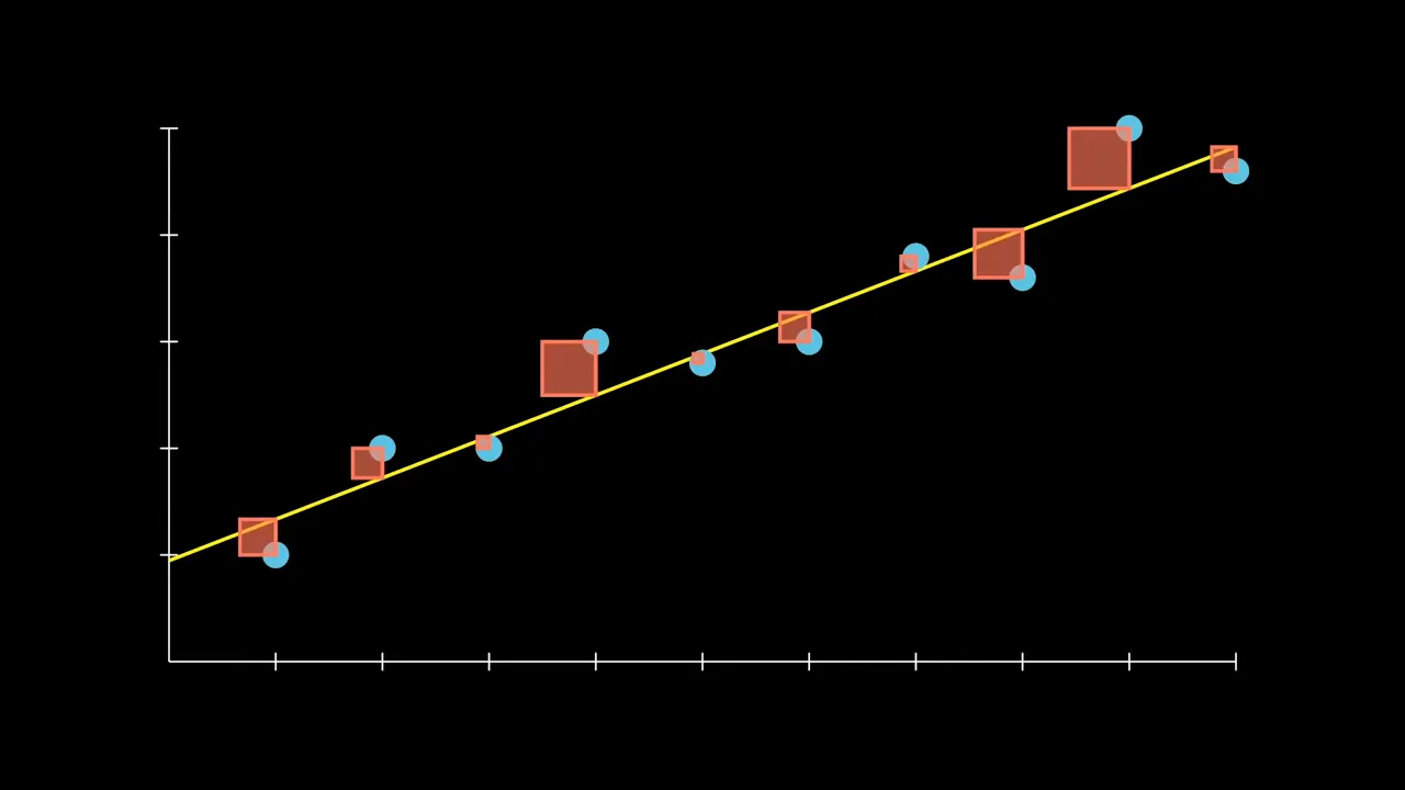
The video then moves from abstraction to data. Several observations are plotted as scattered points in the plane, showing the kind of input from which a regression line will be estimated.
A dashed straight line is drawn through the point cloud and called the regression line. The narrator names the least squares method as the basis for choosing that line.
To explain what least squares is doing, the clip marks one observed point as 'actual' and the corresponding point on the line as 'estimated'. The vertical gap between them is labeled 'errors', and similar vertical gaps are shown for other points.
The fitting objective is then stated plainly: choose the line so that these errors are as small as possible. On screen, the phrase 'minimize errors' reinforces that this is the central criterion.
Finally, the abstract X-axis is given a concrete interpretation by introducing study time as the independent variable, setting up a real-world example that is not yet solved within this segment.
The clip opens on a coordinate plane whose vertical axis is the dependent variable and whose horizontal axis is study time. The narrator specializes the vertical label to grades or GPA, setting up a regression example in which one quantity is predicted from another.
An upward-sloping dashed line is drawn across the graph. This visual encodes the claim that as study time increases, grades increase, and the on-screen label + positive relationship names the pattern.
The video then introduces the algebraic form of the model. The equation is built as y^=b0+b1X, with y^ identified as estimated grades and X identified as study time.
The constant term b0 is isolated and linked to the point where the line meets the vertical axis. The narration states that b0 is derived mathematically and is the y-intercept.
Next, the coefficient b1 is attached to the steepness of the line. Because the drawn line rises, the slope is presented as +b1, and the narrator notes that the detailed derivation will come in a later video.
The example is then contrasted by changing the horizontal variable from study time to time on Facebook. The dashed line now slopes downward, and the label - negative relationship indicates that more Facebook time corresponds to lower grades.
The regression equation is rewritten for this second case as y^=b0−b1X. The left-hand side still estimates grades, but the sign in front of the slope term has changed to reflect the downward direction of the line.
The intercept b0 remains the y-intercept in this negative example as well. The video emphasizes that it is still a calculated value located where the line crosses the vertical axis.
The slope is now identified as −b1 because the line is downward sloping. This is a notation choice in the clip: b1 is treated as a magnitude and the minus sign is written explicitly in the equation.
In the closing section, the specific labels give way to the general roles of the variables. X is called the independent variable, described as what we control, manipulate, or change, while y is called the dependent variable, described as the outcome.
The video returns to the study-time example to consolidate the idea: study time is the independent variable, and grades depend on how much one studies. The final message is that a linear regression equation summarizes how an outcome changes with a chosen predictor.
The clip begins with a brief blank white frame before any content appears.
A static regression board fills the screen. On the left is a scatter plot with axes labeled x and y, five plotted points, a dashed fitted line, and guide lines marking the point (3,4). On the right is a table listing the data pairs (1,2),(2,4),(3,5),(4,4),(5,5), their means xˉ=3 and yˉ=4, and the computed columns x−xˉ, y−yˉ, (x−xˉ)2, and (x−xˉ)(y−yˉ).
Below the table, the slope is written as b1=106=.6=∑(x−xˉ)2∑(x−xˉ)(y−yˉ). To the lower left, the intercept is found by substituting the mean point into the line equation: 4=b0+.6(3), then 4=b0+1.8, and finally 2.2=b0.
A yellow summary box states the completed coefficients and fitted model: b0=2.2, b1=.6, and y^=2.2+.6x. The narration at this stage says the material looks complicated but will be explained step by step in the next video.
The worksheet fades away to a white screen, ending the mathematical portion of the excerpt.
A title card appears reading 'Introduction to regression', with 'David Longstreet' and 'www.MyBookSucks.Com' beneath it.
An animated book-and-arrow logo moves into the upper-left corner of the title slide.
A red diagonal stamp reading 'PARTY MORE STUDY LESS' overlays the title card, and the clip ends without introducing further mathematics.
Knowledge cards
01
Regression setup with X and Y axes
The video introduces regression using a two-variable coordinate system. The horizontal axis is X and is identified as the independent variable; the vertical axis is Y and is identified as the dependent variable. A straight line is then used to represent the relationship between them.
02
Positive relationship
A positive relationship is shown when the independent variable increases and the dependent variable also increases. Visually, this corresponds to an upward-sloping line and is labeled '+ Positive'.
03
Negative relationship
A negative relationship is shown when the independent variable increases but the dependent variable decreases. Visually, this corresponds to a downward-sloping line and is labeled '- Negative'.
04
Linear regression means a straight line
The narrator emphasizes that in linear regression the key word is 'line'. Although curved fits are mentioned as possible in a broader context, this topic is restricted to fitting a straight line to the data.
05
Observations and the regression line
To conduct regression, the video first plots multiple observations as scattered points. It then draws a straight line through the cloud of points and calls this the regression line, saying it is based on the least squares method.
06
Errors as actual-versus-estimated differences
The clip explains error by comparing an observed point labeled 'actual' with the corresponding point on the fitted line labeled 'estimated'. The vertical gap between them is labeled 'errors', and the stated goal is to minimize these errors or make them as small as possible.
07
Concrete example begins with study time
Near the end, the abstract independent variable is replaced by a real example: study time is placed on the x-axis as the independent variable. This starts a concrete application, but no numerical regression result is shown in the clip.
08
Positive relationship in regression
The study-time example shows grades (GPA) on the vertical axis and study time on the horizontal axis. The dashed line rises from left to right, and the video labels this pattern + positive relationship.
09
Linear regression equation with positive slope
The clip builds the equation y^=b0+b1X, where y^ is estimated grades, b0 is the y-intercept, and +b1 is the positive slope when X is study time.
y^=b0+b1X
10
Meaning of b0
The video marks a point on the vertical axis as b0 and states that this constant term is derived mathematically and equals the intercept of the line.
b0=y-intercept
11
Negative relationship in regression
After switching the X-axis to time on Facebook, the dashed line falls from left to right. The video labels this - negative relationship and says grades go down as Facebook time increases.
12
Linear regression equation with negative slope
For the Facebook-time example, the equation becomes y^=b0−b1X. The intercept remains b0, but the slope is presented as −b1 because the line falls.
y^=b0−b1X
13
Independent and dependent variables
The closing summary relabels the axes as independent variable and dependent variable. The narration describes X as what we control, manipulate, or change, and y as the outcome.
14
Linear regression fitted-line form
The video defines the fitted model as a straight line y^=b0+b1x, where b0 is the intercept and b1 is the slope. In the example, the numerical line is y^=2.2+0.6x, and the dashed line on the scatter plot represents this fitted relationship.
y^=b0+b1x
15
Slope formula shown in the example
The slope is computed from centered data using the displayed formula b1=∑(x−xˉ)2∑(x−xˉ)(y−yˉ). The table supplies the needed totals, giving b1=6/10=0.6.
b1=∑(x−xˉ)2∑(x−xˉ)(y−yˉ)
16
Intercept from the mean point
After finding the slope, the example substitutes the sample means (xˉ,yˉ)=(3,4) into the regression equation: 4=b0+0.6(3). Solving yields b0=2.2.
4=b0+.6(3)⇒2.2=b0
17
Five-point worked regression example
Using the data pairs (1,2),(2,4),(3,5),(4,4),(5,5), the clip computes the means, centered deviations, squared deviations, and cross-products, then derives the fitted line y^=2.2+0.6x.
y^=2.2+.6x
18
Title-card transition after the math board
From 9 to 18 seconds the mathematical worksheet disappears and a title slide appears reading 'Introduction to regression', followed by branding elements and the slogan 'PARTY MORE STUDY LESS'. No new mathematics is introduced in this interval.
Detailed learning notes
Explore conditions, steps and evidence. Supplementary explanations are labeled separately from content shown in the video.
Symbols · 16
X
Clear evidence
Shown in the video
Evidence
Diagram
Observation
A horizontal blue axis is drawn and labeled X.
Audio
Observation
The narrator says there is an x variable and identifies the independent variable as being on the x-axis.
Symbol
X
Meaning
horizontal axis representing the independent variable in the regression setup
Domain
real-valued explanatory quantity; no explicit domain is stated
Y
Clear evidence
Shown in the video
Evidence
Diagram
Observation
A vertical green axis is drawn and labeled Y.
Audio
Observation
The narrator says there is a y variable and identifies the dependent variable as being on the y-axis.
Symbol
Y
Meaning
vertical axis representing the dependent variable in the regression setup
Domain
real-valued response quantity; no explicit domain is stated
X
Clear evidence
Shown in the video
Evidence
Diagram
Observation
The horizontal axis is labeled X and is used for study time, then time on facebook, then independent variable.
Symbol
X
Meaning
Independent variable or predictor in the regression examples; concretely study time or time on Facebook.
Domain
Real-valued explanatory quantity shown on the horizontal axis.
y
Clear evidence
Shown in the video
Evidence
Diagram
Observation
The vertical axis is labeled y and is used for dependent variable, grades (GPA), and grades.
Symbol
y
Meaning
Dependent variable or outcome in the regression examples; concretely grades or GPA.
Domain
Real-valued response quantity shown on the vertical axis.
y^
Clear evidence
Shown in the video
Evidence
Formula
Observation
The equation begins with y^ = ...
Audio
Observation
In this case, y hat is estimated grades.
Diagram
Observation
An arrow labels y^ as estimated grades.
Symbol
y^
Meaning
Estimated value of the dependent variable; in these examples, estimated grades.
Domain
Predicted response value produced by the regression line.
b0
Clear evidence
Shown in the video
Evidence
Formula
Observation
The displayed equations contain b0 as the constant term.
Audio
Observation
B naught we derive mathematically, and it is the y intercept.
Diagram
Observation
A point on the vertical axis is labeled b0 and y intercept.
Symbol
b0
Meaning
Y-intercept of the regression line; a calculated constant term.
Domain
Constant coefficient in the linear model.
b1
Clear evidence
Shown in the video
Evidence
Formula
Observation
The displayed equations contain b1 multiplying X.
Audio
Observation
B one we also derive mathematically... and it's the slope of the line.
Diagram
Observation
The term + b1 is labeled slope in the positive example, and - b1 is labeled slope in the negative example.
Uncertainties
The video uses b1 as a magnitude and writes the negative example as b0−b1X rather than b0+b1X with b1<0.
Symbol
b1
Meaning
Slope magnitude associated with the X term; the actual line slope is +b1 in the first example and -b_1 in the second.
Domain
Coefficient multiplying the independent variable.
y^
Clear evidence
Shown in the video
Evidence
Formula
Observation
The fitted-line equation is shown as y^=b0+b1x, and a numerical instance y^=2.2+.6x appears in the yellow box.
Symbol
y^
Meaning
Predicted or fitted value of the response variable from the regression line.
Domain
Real-valued response scale
b0
Clear evidence
Shown in the video
Evidence
Formula
Observation
The intercept symbol b0 appears in the equation y^=b0+b1x and in the solved expression 2.2=b0. The yellow box states b0=2.2.
Symbol
b0
Meaning
Regression intercept, the constant term in the fitted linear model.
Domain
Real number
b1
Clear evidence
Shown in the video
Evidence
Formula
Observation
The slope symbol b1 appears in y^=b0+b1x, in the substitution 4=b0+.6(3), and in the formula b1=106=.6=∑(x−xˉ)2∑(x−xˉ)(y−yˉ). The yellow box states b1=.6.
Symbol
b1
Meaning
Regression slope, the coefficient multiplying x in the fitted line.
Domain
Real number
x
Clear evidence
Shown in the video
Evidence
Formula
Observation
The table header uses x, and the plotted horizontal axis is labeled x. The values listed are 1,2,3,4,5 with mean 3.
Diagram
Observation
The scatter plot shows five data points positioned by their x coordinates on the horizontal axis.
Symbol
x
Meaning
Explanatory or predictor variable in the regression example.
Domain
Observed numeric data values
y
Clear evidence
Shown in the video
Evidence
Formula
Observation
The table header uses y, and the plotted vertical axis is labeled y. The values listed are 2,4,5,4,5 with mean 4.
Diagram
Observation
The scatter plot shows five data points positioned by their y coordinates on the vertical axis.
Symbol
y
Meaning
Response or dependent variable in the regression example.
Domain
Observed numeric data values
Knowledge points · 17
Regression as a line relating two variables
Clear evidence
Shown in the video
Evidence
Audio
Observation
The narrator introduces the tutorial as an introduction to regression and says they try to form a relationship between two variables and draw a straight line.
Diagram
Observation
Title slide reads 'Introduction to regression'; then a coordinate system with X and Y axes appears, followed by a dashed upward-sloping line labeled 'Line'.
Definition
Explanation
The video presents regression as a way to relate an independent variable on the X-axis to a dependent variable on the Y-axis by drawing a line between them. In this introductory segment, the emphasized case is a straight line.
Formula
Conditions
Two variables are considered: one independent and one dependent.
The displayed example uses a straight line rather than a curve.
Axis assignment for independent and dependent variables
Clear evidence
Shown in the video
Evidence
Audio
Observation
The narrator states that the independent variable is on the x-axis and the dependent variable is on the y-axis.
Diagram
Observation
The horizontal axis is labeled 'independent variable' and the vertical axis is labeled 'dependent variable'.
Definition
Explanation
In the regression graph shown here, the explanatory or independent variable is placed on the horizontal axis and the response or dependent variable is placed on the vertical axis.
Formula
Conditions
The graph is a standard two-variable scatterplot-style coordinate display.
Positive relationship between variables
Clear evidence
Shown in the video
Evidence
Audio
Observation
The narrator says that if the independent variable increases and the dependent variable increases as well, there is a positive relationship.
Diagram
Observation
An upward-sloping dashed line is labeled '+ Positive'.
Animation
Observation
A point moves right along the X-axis while another point moves upward along the Y-axis.
Definition
Explanation
A positive relationship is defined verbally and visually as co-movement in the same direction: when the independent variable increases, the dependent variable also increases. The corresponding line slopes upward from left to right.
Formula
Conditions
Both variables are treated as increasing quantities in the displayed example.
Prerequisites
Axis assignment for independent and dependent variables
Negative relationship between variables
Clear evidence
Shown in the video
Evidence
Audio
Observation
The narrator says that if the independent variable increases and the dependent variable decreases, there is a negative relationship.
Diagram
Observation
A downward-sloping dashed line is labeled '- Negative'.
Animation
Observation
A point moves right along the X-axis while another point moves downward along the Y-axis.
Definition
Explanation
A negative relationship is defined verbally and visually as opposite movement: when the independent variable increases, the dependent variable decreases. The corresponding line slopes downward from left to right.
Formula
Conditions
Both variables are treated as changing quantities in the displayed example.
Prerequisites
Axis assignment for independent and dependent variables
Meaning of 'linear' in linear regression
Clear evidence
Shown in the video
Evidence
Audio
Observation
The narrator says, 'In linear regression we try to make a line,' and emphasizes that the key is on 'line,' meaning a straight line.
Diagram
Observation
The label 'Linear Regression' appears next to the dashed straight line.
Definition
Explanation
The video defines linear regression at this level by stressing the word 'line': the fitted object is a straight line. It also notes that curved lines can be used in other contexts, but this topic is about straight lines.
Formula
Conditions
The discussion is restricted to the straight-line case in this tutorial segment.
Prerequisites
Regression as a line relating two variables
Observations plotted for regression
Clear evidence
Shown in the video
Evidence
Audio
Observation
The narrator says that to conduct regression, they take observations and plot more observations randomly.
Diagram
Observation
Multiple colored dots appear scattered across the coordinate plane under the label 'observations'.
Method
Explanation
Regression is introduced operationally by first collecting observations and plotting them as points in the two-variable coordinate system. These plotted points are the data to which a line will later be fitted.
Formula
Conditions
At least two variables are available for each observation.
The points are displayed in a scatterplot-like arrangement.
Prerequisites
Axis assignment for independent and dependent variables
Regression line as a fitted straight line
Clear evidence
Shown in the video
Evidence
Audio
Observation
The narrator says they try to find a straight line that fits all these different points and calls it the regression line.
Diagram
Observation
A dashed straight line passes through the cloud of points and is labeled 'Regression Line'.
Definition
Explanation
The regression line is the straight line chosen to fit the plotted observations. In this clip it is presented visually as a single dashed line running through the point cloud.
Formula
Conditions
There is a set of plotted observations in the plane.
The fit is constrained to a straight line in this segment.
Prerequisites
Observations plotted for regression
Meaning of 'linear' in linear regression
Least squares method named as basis of the regression line
Clear evidence
Shown in the video
Evidence
Audio
Observation
The narrator says the regression line is based upon the least squares method.
Diagram
Observation
Text below 'Regression Line' reads 'least squares method'.
Method
Explanation
The video names the least squares method as the basis for the regression line, but it does not yet show the algebraic formula or derivation in this clip.
Formula
Conditions
The line is being fitted to plotted observations.
Prerequisites
Regression line as a fitted straight line
Errors as differences between estimated and actual values
Clear evidence
Shown in the video
Evidence
Audio
Observation
The narrator says they want to minimize the difference between the estimated value and the actual value, and calls these errors.
Diagram
Observation
One point is labeled 'estimated' on the line and another 'actual' below it, joined by a vertical dashed segment labeled 'errors'.
Animation
Observation
Vertical dashed segments are drawn from multiple points to the regression line.
Definition
Explanation
The clip defines error visually as the vertical discrepancy between an observed point and the fitted line. The point on the line is labeled 'estimated' and the observed point is labeled 'actual'; the connecting vertical segment is labeled 'errors'.
Formula
Conditions
A fitted line has already been drawn.
Each observation is compared to the line at the same horizontal position.
Prerequisites
Regression line as a fitted straight line
Objective of minimizing errors in regression fitting
Clear evidence
Shown in the video
Evidence
Audio
Observation
The narrator repeatedly says the goal is to minimize the errors and make them as small as possible.
Diagram
Observation
The text 'minimize errors' appears beneath the scatterplot with vertical error segments.
Method
Explanation
The fitting objective presented here is to choose the line so that the discrepancies between actual observations and estimated values on the line are as small as possible. This is the conceptual statement of the least-squares goal in the clip.
Formula
Conditions
The comparison is between actual observations and estimated values on the fitted line.
Prerequisites
Least squares method named as basis of the regression line
Errors as differences between estimated and actual values
Linear regression equation for estimated grades from study time
Clear evidence
Shown in the video
Evidence
Audio
Observation
In regression, we develop these equations like this.
Formula
Observation
y^=b0+b1X
Formula
Explanation
The video introduces a simple linear regression equation in which the estimated dependent variable is written as a constant plus a slope times the independent variable. In the study-time example, the equation is presented as y^=b0+b1X, where y^ is estimated grades and X is study time.
Formula
y^=b0+b1X
Conditions
Used for a straight-line regression model with one independent variable.
In this example, X denotes study time and y^ denotes estimated grades.
Prerequisites
y^
b0
b1
X
y
Positive relationship between study time and grades
Clear evidence
Shown in the video
Evidence
Audio
Observation
As study time increases, grades should go up. There is a positive relationship.
Diagram
Observation
An upward-sloping dashed line appears with the label + positive relationship.
Definition
Explanation
A positive relationship is illustrated by an upward-sloping line: as the X-variable study time increases, the Y-variable grades increase.
Formula
Conditions
Applies when larger values of the independent variable correspond to larger values of the dependent variable.
Prerequisites
X
y
Derivations and proofs · 4
Directional reasoning from moving variables to line sign
Clear evidence
Shown in the video
Evidence
Audio
Observation
The narrator asks what happens to the dependent variable as the independent variable changes, then distinguishes same-direction movement from opposite-direction movement.
Animation
Observation
First the X-point moves right while the Y-point moves up; later the X-point moves right while the Y-point moves down.
Diagram
Observation
The corresponding lines are labeled '+ Positive' and '- Negative'.
Visual argument
Steps
Expression
Explanation
The video sets up the question by treating the independent variable as changing along the X-axis and asking how the dependent variable responds along the Y-axis.
Justification
This is directly stated in the narration and shown by the animated axis points.
Shown in the video
Expression
Explanation
When both variables move in the same direction, specifically X increases while Y increases, the displayed line slopes upward and is called a positive relationship.
Justification
The animation shows simultaneous rightward and upward motion, and the label '+ Positive' appears on the upward-sloping line.
Shown in the video
Expression
Explanation
When the variables move in opposite directions, specifically X increases while Y decreases, the displayed line slopes downward and is called a negative relationship.
Justification
The second animation shows rightward motion on X with downward motion on Y, and the label '- Negative' appears on the downward-sloping line.
Shown in the video
Conclusion
The clip uses animated co-movement to define positive versus negative relationships by the direction of the resulting straight line.
Deriving the positive-slope regression example from the graph
Clear evidence
Shown in the video
Evidence
Audio
Observation
As study time increases, grades should go up. There is a positive relationship. In regression, we develop these equations like this... B naught... is the y intercept... B one... is the slope of the line, and in this case the slope is positive.
Formula
Observation
y^=b0+b1X
Diagram
Observation
Upward-sloping dashed line with b0 marked at the y-axis and +b1 labeled slope.
Visual argument
Steps
Expression
X=study time,y=grades (GPA)
Explanation
The axes assign study time to the horizontal variable and grades to the vertical variable.
Justification
Directly shown by the axis labels and stated in the audio.
Shown in the video
Expression
as X increases, y increases
Explanation
The upward-sloping dashed line represents a positive relationship between study time and grades.
Justification
Stated in the audio and shown by the rising line labeled + positive relationship.
Shown in the video
Expression
y^=b0+b1X
Explanation
The regression line is written in slope-intercept form, with estimated grades on the left and a constant plus slope times study time on the right.
Justification
Displayed formula and spoken explanation introduce the regression equation.
Shown in the video
Expression
b0=y-intercept
Explanation
The constant term is identified as the point where the line meets the vertical axis.
Justification
Audio states B naught is the y intercept, and the diagram marks b0 on the y-axis.
Shown in the video
Expression
slope=+b1
Explanation
Because the line rises, the slope term is presented as positive b1.
Justification
Audio says the slope is positive, and the diagram labels +b1 as slope.
Shown in the video
Conclusion
For the study-time example, the regression model is y^=b0+b1X with positive slope +b1 and intercept b0.
Deriving the negative-slope regression example from the graph
Clear evidence
Shown in the video
Evidence
Audio
Observation
Now if I change the x-axis to time on Facebook, we see a negative relationship... What we're estimating is still grades... is equal to b naught minus b one times x, where x is time on Facebook... The slope of the line is negative b one because it's downward sloping.
Formula
Observation
y^=b0−b1X
Diagram
Observation
Downward-sloping dashed line with b0 marked at the y-axis and -b_1 labeled slope.
Uncertainties
The video does not explain whether b1 itself is assumed positive or merely denotes a magnitude.
Visual argument
Steps
Expression
X=time on facebook,y=grades
Explanation
The horizontal variable is changed from study time to time on Facebook while the vertical variable remains grades.
Justification
Axis relabeling is shown visually and stated in the audio.
Shown in the video
Expression
as X increases, y decreases
Explanation
The downward-sloping dashed line represents a negative relationship between Facebook time and grades.
Justification
Audio states more time on Facebook makes grades go down, and the diagram labels - negative relationship.
Shown in the video
Expression
y^=b0−b1X
Explanation
The regression equation is rewritten with a minus sign before the slope term.
Justification
Displayed formula and spoken explanation give b naught minus b one times x.
Shown in the video
Expression
b0=y-intercept
Explanation
The intercept remains the point where the line crosses the vertical axis.
Justification
Audio repeats that B naught is still the y intercept, and the diagram marks b0 on the y-axis.
Shown in the video
Expression
slope=−b1
Explanation
Because the line falls, the slope is identified as negative b1.
Justification
Audio explicitly says the slope of the line is negative b one because it is downward sloping.
Shown in the video
Conclusion
For the Facebook-time example, the regression model is y^=b0−b1X with intercept b0 and negative slope −b1.
Worked derivation of the fitted line from the displayed table
Clear evidence
Shown in the video
Evidence
Formula
Observation
The table lists (x,y)=(1,2),(2,4),(3,5),(4,4),(5,5) with means 3 and 4.
Formula
Observation
The deviation columns show x−xˉ=(−2,−1,0,1,2) and y−yˉ=(−2,0,1,0,1).
Formula
Observation
The squared-deviation column shows (4,1,0,1,4) totaling 10.
Formula
Observation
The cross-product column shows (4,0,0,0,2) totaling 6.
Formula
Observation
The slope line reads b1=106=.6=∑(x−xˉ)2∑(x−xˉ)(y−yˉ).
Formula
Observation
The intercept line reads 4=b0+.6(3), then 4=b0+1.8, then −1.8, then 2.2=b0.
Numerical verification
Steps
Expression
(x,y)=(1,2),(2,4),(3,5),(4,4),(5,5)
Explanation
Read the five paired observations from the table.
Justification
Directly visible in the displayed data rows.
Shown in the video
Expression
xˉ=3,yˉ=4
Explanation
Identify the sample means shown at the bottom of the table.
Justification
The row labeled mean gives these values explicitly.
Shown in the video
Expression
x−xˉ=(−2,−1,0,1,2),y−yˉ=(−2,0,1,0,1)
Explanation
Compute the centered values for each observation.
Justification
These entries are shown in the deviation columns of the table.
Shown in the video
Expression
∑(x−xˉ)2=4+1+0+1+4=10
Explanation
Sum the squared deviations of x.
Justification
The squared-deviation column and its total are displayed.
Shown in the video
Expression
∑(x−xˉ)(y−yˉ)=4+0+0+0+2=6
Explanation
Sum the cross-products of centered x and y.
Justification
The cross-product column and its total are displayed.
Shown in the video
Expression
b1=106=.6
Explanation
Form the slope as the ratio of the two totals.
Justification
The displayed formula equates this ratio to ∑(x−xˉ)2∑(x−xˉ)(y−yˉ).
Shown in the video
Expression
4=b0+.6(3)
Explanation
Substitute the mean point (xˉ,yˉ)=(3,4) and the slope 0.6 into the regression equation.
Justification
This substitution is written explicitly on screen.
Shown in the video
Expression
4=b0+1.8⇒2.2=b0
Explanation
Solve for the intercept by subtracting 1.8 from both sides.
Justification
The intermediate arithmetic and final result are shown in the lower-left derivation.
Shown in the video
Expression
y^=2.2+.6x
Explanation
Write the fitted line using the computed coefficients.
Justification
The yellow summary box states b0=2.2, b1=.6, and y^=2.2+.6x.
Shown in the video
Conclusion
The displayed example derives the fitted regression line y^=2.2+0.6x from the five data pairs by first computing the slope from centered sums and then solving for the intercept using the mean point.
Worked examples · 4
Study time introduced as an example independent variable
Approximate timing
Shown in the video
Evidence
Audio
Observation
The narrator says, 'Now let's imagine I put study time on the x-axis or make that my independent variable.'
Diagram
Observation
The generic axis label is replaced by 'study time' on the horizontal axis near the end of the clip.
Uncertainties
No numerical data, fitted equation, or completed worked solution is shown before the clip ends.
Problem
Introduce a concrete explanatory variable for the regression setup by placing study time on the x-axis.
Given
The general regression coordinate system is already established.
The horizontal axis represents the independent variable.
Goal
Replace the abstract independent variable with a concrete example variable, study time.
Steps
Expression
Explanation
The narrator transitions from the abstract X-axis to a named real-world variable, saying to imagine putting study time on the x-axis.
Justification
This is explicitly spoken in the audio.
Shown in the video
Expression
Explanation
The horizontal axis label changes to 'study time', indicating that this variable is being used as the independent variable in the example.
Justification
The on-screen axis label visibly changes near the end of the clip.
Shown in the video
Answer
The clip begins a concrete example by assigning study time to the independent-variable axis, but it does not complete any calculation within the provided duration.
Verification
Verification is limited to confirming the spoken transition and the visible axis relabeling; no numeric check is possible because no full example is completed.
Positive regression example: study time predicts grades
Clear evidence
Shown in the video
Evidence
Audio
Observation
And the dependent variable becomes grades or GPA. As study time increases, grades should go up. There is a positive relationship. In regression, we develop these equations like this... where x is study time.
Formula
Observation
y^=b0+b1X
Diagram
Observation
Graph with y-axis grades (GPA), x-axis study time, upward dashed line, b0 at intercept, +b1 labeled slope.
Problem
Model how grades depend on study time using a straight-line regression equation.
Given
X is study time.
y is grades (GPA).
The relationship is positive.
Goal
Write the regression equation and identify the intercept and slope.
Steps
Expression
y^=b0+b1X
Explanation
Use the linear regression form with estimated grades on the left and study time on the right.
Justification
The video introduces this exact equation for the example.
Shown in the video
Expression
b0=y-intercept
Explanation
Identify the constant term as the intercept on the grades axis.
Justification
Audio and diagram both label b0 as the y intercept.
Shown in the video
Expression
slope=+b1
Explanation
Identify the coefficient of X as the positive slope because the line rises.
Justification
Audio states the slope is positive and the diagram labels +b1 as slope.
Shown in the video
Answer
y^=b0+b1X, with b0 as the y-intercept and slope +b1.
Verification
The upward-sloping dashed line and the label + positive relationship match the stated equation structure.
Negative regression example: time on Facebook predicts grades
Clear evidence
Shown in the video
Evidence
Audio
Observation
Now if I change the x-axis to time on Facebook, we see a negative relationship... What we're estimating is still grades... is equal to b naught minus b one times x, where x is time on Facebook.
Formula
Observation
y^=b0−b1X
Diagram
Observation
Graph with y-axis grades, x-axis time on facebook, downward dashed line, b0 at intercept, -b_1 labeled slope.
Problem
Model how grades depend on time on Facebook using a straight-line regression equation.
Given
X is time on Facebook.
y is grades.
The relationship is negative.
Goal
Write the regression equation and identify the intercept and slope.
Steps
Expression
y^=b0−b1X
Explanation
Use the same regression structure but with a minus sign before the slope term.
Justification
The video displays and speaks this equation for the Facebook example.
Shown in the video
Expression
b0=y-intercept
Explanation
Keep the constant term as the intercept on the grades axis.
Justification
Audio says B naught is still the y intercept, and the diagram marks it on the y-axis.
Shown in the video
Expression
slope=−b1
Explanation
Identify the slope as negative because the line falls as X increases.
Justification
Audio explicitly states the slope is negative b one because it is downward sloping.
Shown in the video
Answer
y^=b0−b1X, with b0 as the y-intercept and slope −b1.
Verification
The downward-sloping dashed line and the label - negative relationship match the stated equation structure.
Five-point linear regression example
Clear evidence
Shown in the video
Evidence
Formula
Observation
The table contains the five pairs (1,2),(2,4),(3,5),(4,4),(5,5) and the derived columns needed for regression.
Diagram
Observation
The scatter plot shows these five points together with a dashed fitted line and guide lines through (3,4).
Formula
Observation
The yellow box summarizes the result as b0=2.2, b1=.6, and y^=2.2+.6x.
Problem
Fit a straight-line regression model to the displayed five paired observations and determine the numerical equation of the line.
Given
Data pairs: (1,2),(2,4),(3,5),(4,4),(5,5).
Sample means: xˉ=3, yˉ=4.
Centered sums shown in the table: ∑(x−xˉ)2=10 and ∑(x−xˉ)(y−yˉ)=6.
Goal
Find b1, then b0, and write the fitted equation y^=b0+b1x.
Steps
Expression
b1=106=.6
Explanation
Use the displayed slope formula with the table totals.
Justification
The formula and totals are both visible on screen.
Shown in the video
Expression
4=b0+.6(3)
Explanation
Substitute the mean point and the slope into the regression equation.
Justification
This step is written explicitly in the lower-left derivation.
Shown in the video
Expression
2.2=b0
Explanation
Solve the previous equation for the intercept.
Justification
The arithmetic simplification is shown on screen.
Shown in the video
Expression
y^=2.2+.6x
Explanation
State the final fitted line.
Justification
The yellow summary box displays this exact equation.
Shown in the video
Answer
y^=2.2+0.6x
Verification
The result matches the yellow box values b0=2.2 and b1=.6, and the dashed line on the graph is consistent with a positive-slope fit passing near the mean point (3,4).
Visual events · 11
Title slide and construction of the regression coordinate system
Clear evidence
Shown in the video
Evidence
Diagram
Observation
A title slide reading 'Introduction to regression' gives way to a coordinate system with a blue horizontal X-axis and a green vertical Y-axis.
Animation
Observation
The axes are drawn sequentially, then labeled 'independent variable' and 'dependent variable'.
Objects
title text
horizontal X-axis
vertical Y-axis
axis labels
Changes
The screen changes from a title slide to a blank coordinate plane.
The horizontal axis is drawn first, then the vertical axis.
Text labels identify the axes as independent and dependent variables.
Invariants
The horizontal axis remains associated with X.
The vertical axis remains associated with Y.
Interpretation
This visual sequence establishes the standard two-variable framework used throughout the rest of the clip.
Introduction of a generic regression line
Clear evidence
Shown in the video
Evidence
Diagram
Observation
A dashed upward-sloping line appears across the coordinate plane and is labeled 'Line'.
Animation
Observation
Dashed guide lines connect a point on the X-axis to a point on the Y-axis and then to the sloped line.
Objects
dashed sloped line
guide lines
label 'Line'
Changes
A single straight line is added to the empty coordinate system.
Temporary guide lines illustrate correspondence between axis positions and the line.
Invariants
The line remains straight.
The axes remain fixed in orientation.
Interpretation
The clip visually states that regression is represented here by fitting a straight line between the two variables.
Animation of a positive relationship
Clear evidence
Shown in the video
Evidence
Animation
Observation
A point travels rightward along the X-axis while another point travels upward along the Y-axis.
Diagram
Observation
An upward-sloping dashed line is labeled '+ Positive'.
Objects
moving X-point
moving Y-point
upward-sloping dashed line
label '+ Positive'
Changes
The independent-variable point increases along X.
The dependent-variable point increases along Y.
The line is identified as positive.
Invariants
The X-axis still represents the independent variable.
The Y-axis still represents the dependent variable.
Interpretation
Same-direction movement of the two variables is mapped to an upward-sloping line.
Animation of a negative relationship
Clear evidence
Shown in the video
Evidence
Animation
Observation
A point travels rightward along the X-axis while another point travels downward along the Y-axis.
Diagram
Observation
A downward-sloping dashed line is labeled '- Negative'.
Objects
moving X-point
moving Y-point
downward-sloping dashed line
label '- Negative'
Changes
The independent-variable point increases along X.
The dependent-variable point decreases along Y.
The line is identified as negative.
Invariants
The axes retain the same roles as before.
Interpretation
Opposite-direction movement of the two variables is mapped to a downward-sloping line.
From scattered observations to a fitted regression line
Clear evidence
Shown in the video
Evidence
Diagram
Observation
Multiple colored dots appear under the label 'observations' and then a dashed line is drawn through them labeled 'Regression Line' with 'least squares method' below.
Animation
Observation
Points are added one after another until a scattered cloud is visible, after which the fitted line appears.
Objects
scatter points
label 'observations'
dashed regression line
labels 'Regression Line' and 'least squares method'
Changes
Individual plotted points accumulate into a data cloud.
A single straight line is overlaid through the cloud.
The method name 'least squares method' is displayed.
Invariants
The plot remains in the same X-Y coordinate system.
The fitted object remains a straight line.
Interpretation
This sequence shows regression as fitting one line to many observed paired values.
Visualization of errors and the minimization objective
Clear evidence
Shown in the video
Evidence
Diagram
Observation
One observed point is labeled 'actual', a point on the line is labeled 'estimated', and a vertical dashed connector is labeled 'errors'.
Animation
Observation
Additional vertical dashed segments are drawn from several points to the regression line, and the phrase 'minimize errors' appears.
Objects
actual point
estimated point
vertical dashed error segments
regression line
text 'minimize errors'
Changes
A single vertical discrepancy is highlighted first.
More vertical discrepancies are shown across multiple observations.
The minimization message is added on screen.
Invariants
The regression line stays fixed during this explanation.
Error is shown as a vertical distance at a given horizontal position.
Interpretation
The clip uses vertical gaps between points and the line to explain what least-squares fitting is trying to reduce.
Positive-relationship graph build-up
Clear evidence
Shown in the video
Evidence
Diagram
Observation
A coordinate plane shows y-axis labeled grades (GPA), x-axis labeled study time, an upward dashed line, the text + positive relationship, then the equation y^=b0+b1X with b0 marked on the y-axis and +b1 labeled slope.
Objects
green vertical y-axis
purple horizontal x-axis
upward dashed regression line
equation y^=b0+b1X
point b0 on the y-axis
label +b1 as slope
Changes
Axis labels appear first as dependent variable and study time, then grades (GPA) replaces dependent variable.
The dashed line is drawn upward from left to right.
The equation is built term by term until y^=b0+b1X is complete.
b0 is highlighted at the y-axis intercept and +b1 is highlighted as the slope.
Invariants
The vertical axis continues to represent grades/GPA.
The horizontal axis continues to represent study time.
The line remains straight and upward sloping.
Interpretation
The visual sequence links a rising line to a positive regression relationship and identifies the intercept and slope in the equation.
Negative-relationship graph build-up
Clear evidence
Shown in the video
Evidence
Diagram
Observation
The x-axis changes to time on facebook, the dashed line slopes downward, the text - negative relationship appears, and the equation becomes y^=b0−b1X with b0 at the intercept and -b_1 labeled slope.
Objects
green vertical y-axis
purple horizontal x-axis
downward dashed regression line
equation y^=b0−b1X
point b0 on the y-axis
label -b_1 as slope
Changes
The x-axis label changes from study time to time on facebook.
The dashed line changes from upward sloping to downward sloping.
The equation changes from plus b1X to minus b1X.
The slope annotation changes from +b1 to -b_1.
Invariants
The vertical axis still represents grades.
The intercept remains marked as b0 on the y-axis.
The model remains a straight-line regression equation.
Interpretation
The visual sequence contrasts the earlier positive example by showing that changing the predictor to time on Facebook yields a negative slope.
General variable-role summary
Clear evidence
Shown in the video
Evidence
Diagram
Observation
The axes are relabeled independent variable and dependent variable, with annotations control, manipulate, change near X and outcome near y, then the labels return to study and grades while the equation y^=b0+b1X remains visible.
Objects
x-axis labeled independent variable
y-axis labeled dependent variable
annotations control, manipulate, change
annotation outcome
equation y^=b0+b1X
Changes
Specific example labels are replaced by generic role labels.
Text annotations are added beside the axes to describe each variable's role.
The display then returns toward the study-time example wording.
Invariants
The regression equation remains on screen.
X stays on the horizontal axis and y stays on the vertical axis.
Interpretation
This closing visual generalizes the examples: X is the manipulated input and y is the outcome being estimated.
Static regression worksheet display
Clear evidence
Shown in the video
Evidence
Diagram
Observation
From about 1s to 9s the screen holds a static composite layout: scatter plot on the left, data table upper right, yellow result box above the table, and algebraic derivations below.
Diagram
Observation
The plot contains axes labeled x and y, five plotted points, a dashed regression line, and green/purple guide lines intersecting at (3,4).
Objects
Coordinate axes labeled x and y.
Five scatter points.
Dashed fitted line.
Green horizontal and purple vertical guide lines through (3,4).
Data table with columns x, y, x−xˉ, y−yˉ, (x−xˉ)2, and (x−xˉ)(y−yˉ).
Yellow box with b0=2.2, b1=.6, y^=2.2+.6x.
Lower algebra showing slope and intercept calculations.
Changes
No mathematical content changes during this interval; the board remains static while narration introduces the topic.
Invariants
The displayed data set, means, totals, formulas, and final fitted equation remain unchanged throughout the interval.
Interpretation
The visual layout functions as a worked regression board: the graph gives geometric intuition, the table supplies the raw computations, and the formulas connect those computations to the fitted line.
Transition from worked example to title card
Clear evidence
Shown in the video
Evidence
Animation
Observation
Around 9s the regression board fades out to white.
Caption evidence
Observation
By about 10s a title card reads 'Introduction to regression' with 'David Longstreet' and 'www.MyBookSucks.Com'.
Animation
Observation
Around 11s to 12s a book-and-arrow logo animates into the upper-left area.
Animation
Observation
Around 14s to 15s a red diagonal stamp 'PARTY MORE STUDY LESS' appears across the title card.
Objects
Blank white transition frame.
Title text 'Introduction to regression'.
Author/site text 'David Longstreet' and 'www.MyBookSucks.Com'.
Animated book-and-arrow logo.
Red diagonal slogan stamp 'PARTY MORE STUDY LESS'.
Changes
The mathematical worksheet disappears.
A title slide replaces it.
The logo animates in.
The red slogan stamp appears diagonally over the slide.
Invariants
No new mathematical notation or derivation is introduced after the transition.
Interpretation
This segment is branding and title information rather than additional mathematics; it marks the end of the excerpted worked example view.
Misconceptions · 3
Assuming all regression must be curved or that linear regression includes curves by default
Clear evidence
Shown in the video
Evidence
Audio
Observation
The narrator says, 'You can also do curved lines, but for this topic it's all straight lines.'
Misconception
A learner may think the discussion allows arbitrary curved fits because the narrator mentions curved lines.
Clarification
The video explicitly limits this topic to straight-line fitting: curved relationships exist, but the present lesson is about linear regression with a straight line.
Overgeneralizing the displayed error picture into a full formal theory
Approximate timing
Derived from the video
Evidence
Diagram
Observation
Errors are drawn only as vertical dashed segments between observations and the regression line.
Audio
Observation
The narrator describes error as the difference between estimated and actual values without stating a general geometric rule beyond this display.
Uncertainties
The clip does not discuss alternative residual geometries or formal definitions beyond the shown vertical distances.
Misconception
A learner may infer from this clip alone that the video has fully defined all aspects of residuals in regression.
Clarification
What is actually shown here is an introductory visual model: error is represented as the vertical gap between an observed point and the fitted line, and the goal is to minimize those gaps.
Sign convention for the slope term
Approximate timing
Supplementary explanation
Evidence
Formula
Observation
The negative example is written as y^=b0−b1X rather than y^=b0+b1X with b1<0.
Audio
Observation
The slope of the line is negative b one because it's downward sloping.
Uncertainties
This is an analyst clarification about notation convention, not an explicit warning given in the video.
Misconception
One might assume the symbol b1 always denotes the signed slope itself.
Clarification
In this video, b1 is treated as a magnitude and the sign is written separately: +b1 for the upward example and -b_1 for the downward example.
Concept relations · 16
Axis assignment for independent and dependent variables → Regression as a line relating two variables
Clear evidence
Shown in the video
Evidence
Audio
Observation
The narrator first names the x and y variables and their axis placement, then says they try to form a relationship and draw a line.
Diagram
Observation
The axes appear before the generic line.
Prerequisite
Explanation
The clip uses the independent/dependent axis assignment as the setup needed before introducing regression as a line relating the two variables.
Regression as a line relating two variables → Positive relationship between variables
Clear evidence
Shown in the video
Evidence
Audio
Observation
After introducing a general relationship, the narrator distinguishes same-direction and opposite-direction cases.
Diagram
Observation
The generic line idea is followed by separate '+ Positive' and '- Negative' displays.
Contains
Explanation
The general idea of relating two variables by a line is specialized here into the positive case.
Regression as a line relating two variables → Negative relationship between variables
Clear evidence
Shown in the video
Evidence
Audio
Observation
The narrator contrasts the negative case with the earlier positive case.
Diagram
Observation
A downward-sloping line labeled '- Negative' replaces the earlier upward-sloping example.
Contains
Explanation
The same general regression relationship framework is also specialized into the negative case.
Regression as a line relating two variables → Meaning of 'linear' in linear regression
Clear evidence
Shown in the video
Evidence
Audio
Observation
The narrator says that in linear regression the key is on 'line' and that this topic is all straight lines.
Diagram
Observation
The label changes to 'Linear Regression' beside the straight line.
Special case
Explanation
Linear regression is presented as the straight-line special case of the broader regression idea introduced earlier.
Observations plotted for regression → Regression line as a fitted straight line
Clear evidence
Shown in the video
Evidence
Audio
Observation
The narrator says they take observations and then try to find a line that fits all these different points.
Animation
Observation
Scattered points appear first, and only afterward is the regression line drawn through them.
Prerequisite
Explanation
The plotted observations are required before the regression line can be discussed as a fit to those points.
Least squares method named as basis of the regression line → Regression line as a fitted straight line
Clear evidence
Shown in the video
Evidence
Audio
Observation
The narrator says the regression line is based upon the least squares method and then explains minimizing errors.
Diagram
Observation
'least squares method' appears with the regression line, followed by error segments and 'minimize errors'.
Proof dependency
Explanation
Within the clip’s explanation, the named least-squares method is what justifies how the regression line is chosen.
Errors as differences between estimated and actual values → Objective of minimizing errors in regression fitting
Clear evidence
Shown in the video
Evidence
Diagram
Observation
The terms 'estimated', 'actual', and 'errors' are introduced before the phrase 'minimize errors' appears.
Audio
Observation
The narrator first defines the difference between estimated and actual values, then states the goal of minimizing those errors.
Prerequisite
Explanation
The clip first identifies what the errors are, then states that the fitting objective is to minimize them.
Positive relationship between variables → Negative relationship between variables
Clear evidence
Shown in the video
Evidence
Audio
Observation
The narrator explicitly contrasts same-direction movement with opposite-direction movement.
Diagram
Observation
Upward and downward sloping lines are shown in succession with '+ Positive' and '- Negative' labels.
Contrast
Explanation
The two concepts are presented as opposite directional patterns between the independent and dependent variables.
Positive relationship between study time and grades → Negative relationship between time on Facebook and grades
Clear evidence
Shown in the video
Evidence
Audio
Observation
Now if I change the x-axis to time on Facebook, we see a negative relationship.
Diagram
Observation
The graph switches from an upward line labeled + positive relationship to a downward line labeled - negative relationship.
Contrast
Explanation
The video directly contrasts a positive regression relationship with a negative one by changing the X-variable and reversing the slope direction.
X → Linear regression equation for estimated grades from study time
Clear evidence
Shown in the video
Evidence
Formula
Observation
y^=b0+b1X
Audio
Observation
where x is study time
Application
Explanation
The independent variable X is inserted into the regression equation as the predictor term.
y^ → Linear regression equation for estimated grades from study time
Clear evidence
Shown in the video
Evidence
Formula
Observation
y^=b0+b1X
Audio
Observation
y hat is estimated grades
Application
Explanation
The symbol y^ is the left-hand side of the regression equation and denotes the estimated outcome.
Independent and dependent variables in regression → X
Clear evidence
Shown in the video
Evidence
Audio
Observation
The X is the independent variable. The Y is the dependent variable.
Diagram
Observation
Axes are relabeled independent variable and dependent variable.
Contains
Explanation
The definition of independent and dependent variables assigns the role of independent variable to X.
Find an answer · 15
How does this video introduce regression as a line relating two variables?
Clear evidence
Shown in the video
Evidence
Audio
Observation
The narrator introduces regression as forming a relationship between two variables and drawing a straight line.
Diagram
Observation
A dashed line labeled 'Line' appears on the coordinate plane.
Knowledge points
Regression as a line relating two variables
Axis assignment for independent and dependent variables
Where are the independent and dependent variables placed on the graph?
Clear evidence
Shown in the video
Evidence
Audio
Observation
The narrator states that the independent variable is on the x-axis and the dependent variable is on the y-axis.
Diagram
Observation
Axis labels read 'independent variable' and 'dependent variable'.
Knowledge points
Axis assignment for independent and dependent variables
What is the difference between a positive and a negative relationship in this regression introduction?
Clear evidence
Shown in the video
Evidence
Audio
Observation
The narrator defines positive and negative relationships by whether the variables move in the same or opposite directions.
Animation
Observation
Rightward X-motion is paired first with upward Y-motion and then with downward Y-motion.
Knowledge points
Positive relationship between variables
Negative relationship between variables
Why does the video stress the word 'line' in linear regression?
Clear evidence
Shown in the video
Evidence
Audio
Observation
The narrator emphasizes that in linear regression the key is on 'line' and says this topic is all straight lines.
Diagram
Observation
The label 'Linear Regression' appears next to a straight dashed line.
Knowledge points
Meaning of 'linear' in linear regression
How is the regression line obtained from plotted observations in this clip?
Clear evidence
Shown in the video
Evidence
Audio
Observation
The narrator says they take observations, plot them, and try to find a straight line that fits all the points.
Animation
Observation
Scattered points appear first, then a dashed regression line is drawn through them.
Knowledge points
Observations plotted for regression
Regression line as a fitted straight line
Least squares method named as basis of the regression line
What does the video mean by errors between estimated and actual values?
Clear evidence
Shown in the video
Evidence
Diagram
Observation
Vertical dashed segments connect 'actual' points to 'estimated' points on the line and are labeled 'errors'.
Audio
Observation
The narrator says the goal is to minimize the difference between estimated and actual values.
Knowledge points
Errors as differences between estimated and actual values
Objective of minimizing errors in regression fitting
Does the clip begin a concrete example using study time as the independent variable?
Approximate timing
Shown in the video
Evidence
Audio
Observation
The narrator says to imagine putting study time on the x-axis as the independent variable.
Diagram
Observation
The horizontal axis label changes to 'study time'.
Uncertainties
The example is only introduced and not worked out within the clip.
Knowledge points
Study time introduced as an example independent variable
What does y^ mean in the regression equation?
Clear evidence
Shown in the video
Evidence
Audio
Observation
In this case, y hat is estimated grades.
Formula
Observation
y^=b0+b1X
Knowledge points
y^
Linear regression equation for estimated grades from study time
What is b0 in the displayed regression line?
Clear evidence
Shown in the video
Evidence
Audio
Observation
B naught we derive mathematically, and it is the y intercept.
Diagram
Observation
b0 is marked on the y-axis and labeled y intercept.
Knowledge points
b0
Linear regression equation for estimated grades from study time
Why is the slope written as -b_1 in the Facebook-time example?
Clear evidence
Shown in the video
Evidence
Audio
Observation
The slope of the line is negative b one because it's downward sloping, negative relationship.
Formula
Observation
y^=b0−b1X
Knowledge points
b1
Negative relationship between time on Facebook and grades
Negative regression example: time on Facebook predicts grades
How does the video distinguish independent and dependent variables?
Clear evidence
Shown in the video
Evidence
Audio
Observation
The X is the independent variable... The Y is the dependent variable... the dependent variable is the outcome.
Diagram
Observation
Annotations control, manipulate, change, and outcome appear beside the axes.
Knowledge points
Independent and dependent variables in regression
X
y
What is the form of the fitted regression line shown in this clip?
Clear evidence
Shown in the video
Evidence
Formula
Observation
The screen shows y^=b0+b1x and y^=2.2+.6x.
Knowledge points
Linear regression fitted-line form
Coverage and review notes
Covered · Title slide and spoken introduction to regression.
Covered · Coordinate axes are drawn and labeled as independent and dependent variables.
Covered · A generic straight line is introduced as the relationship between the two variables.
Covered · The narrator frames the central question of how the dependent variable changes when the independent variable changes.
Covered · Positive relationship is defined and illustrated with an upward-sloping line.
Covered · Brief pause after the positive example before the contrast case begins.
Covered · Negative relationship is defined and illustrated with a downward-sloping line.
Covered · Short transition after the negative example.
Covered · The clip emphasizes that linear regression uses a straight line.
Covered · Transition from the abstract line to data collection for regression.
Covered · Observations are plotted as scattered points.
Covered · A regression line is fitted through the points and named as based on least squares.
Covered · Errors are shown as vertical differences between actual and estimated values, with the goal of minimizing them.
Covered · A concrete example begins by assigning study time to the independent-variable axis.
Covered · Positive study-time example, equation construction, intercept and slope identification.
Covered · Negative Facebook-time example, equation rewrite, intercept and negative slope identification.
Covered · Generic summary of independent and dependent variable roles, then return to the study-time wording.
Covered · Brief blank opening frame before the regression board becomes visible; no mathematical content is presented.
Covered · Main mathematical content: static regression worksheet with scatter plot, data table, slope formula, intercept derivation, and final fitted line.
Covered · Transition to title card and branding animation; no additional mathematics beyond identifying the lesson title.
Reviewed English material v1: card/concept_card "Regression setup with X and Y axes" starting at 0:05 — The video introduces regression using a two-variable coordinate system. The horizontal axis is X and is identified as the independent variable; the vertical axis is Y and is identified as the dependent variable. A straight line is then used to represent the relationship between them.
Reviewed English material v1: knowledge_item/method "Least squares method named as basis of the regression line" from 1:54 to 1:58 — The video names the least squares method as the basis for the regression line, but it does not yet show the algebraic formula or derivation in this clip. The line is being fitted to plotted observations.