Reviewed learning material · Video analysis · EnglishRead the full overview
This 150-second introductory lecture segment explains Economic Order Quantity (EOQ) first as an inventory-management model for minimizing variable inventory costs, then graphically as the order quantity where holding cost and ordering cost intersect, and finally algebraically through the formula EOQ = sqrt((2×(F×S)) / (C×P)). The speaker defines F, S, C, and P, stresses that S must be annual sales in units, and the slide also shows auxiliary formulas for total carrying costs and total restocking costs.
This 150-second lecture segment introduces the Economic Order Quantity formula EOQ = sqrt((2x(FxS))/(C x P)) and defines each variable on a static slide. The speaker explains that C must be expressed as a percentage of inventory value and that annual sales may need to be derived from weekly sales. The same slide then presents two auxiliary formulas: total carrying costs = (Q x CC)/2 and total restocking costs = (F x T)/Q. At 122 seconds the video switches to Example 1 for Jersey Limited and reads the given data, but the clip ends before any numerical solution is computed.
This clip is an introductory worked example on economic order quantity for Jersey Limited. The lecturer first reads the inventory data, then recalls the formula EOQ = sqrt((2 x F x S)/(C x P)), defines each symbol, and substitutes F=100, S=500000, C=0.2, and P=3. He also warns that weekly or monthly demand must be converted to annual units before using the formula. The calculation yields 12 909.95, which is rounded to 12 910 units. The clip ends by interpreting EOQ as the optimal stock level. Although the slide also asks for a reorder point using a 360-day year, delivery time, and safety stock, that second part is not solved in this segment.
This 150-second lecture segment works through an inventory-management example for Jersey Limited. It first recalls the EOQ formula and the computed EOQ of about 12 910 units, then shifts to part 2.2: determining the reorder point. The lecturer defines the reorder level as safety stock plus reorder point, derives daily average usage from 500 000 annual units over a 360-day year, rounds it to 1389 units per day, and multiplies by the 4-day waiting time to obtain a reorder point of 5 556 units.
This video segment explains how to calculate the reorder point and re-order levels in units for a manufacturing company, Jersey Limited. Using given data such as annual sales, delivery time, and desired safety stock, the speaker demonstrates the step-by-step numerical calculations. The core concepts covered include daily average usage, the reorder point formula, and how safety stock is integrated into the total order quantity.
Use the learning inspector for key ideas and moments, or open the reading tabs for the complete notes.
Generated from the video's visuals and explanation; not verbatim speech.
The segment opens by naming the topic: Economic Order Quantity, abbreviated EOQ. The speaker frames it as a model for inventory management rather than as a purely accounting term.
The first definition slide states that EOQ is used to establish optimal inventory levels. The narration adds that the goal is to obtain the correct inventory level a company needs.
A second bullet refines the idea: EOQ is the optimum order quantity a company should hold given production cost, demand rate, and other variables. The stated purpose is to minimize variable inventory costs.
The lesson then switches to a graph with cost on the vertical axis and order quantity on the horizontal axis. One line rises and is labeled "Cost of Holding"; another falls and is labeled "Cost of Ordering".
The speaker explains the tradeoff verbally: as holding cost increases, ordering cost decreases. The reason given is that holding more inventory implies larger orders, and larger orders reduce ordering cost.
The key visual point is the intersection of the two lines. A dashed vertical marker drops to the x-axis at "EOQ", showing that EOQ is located where the two cost trends meet. Above them, a U-shaped "Total Cost" curve illustrates the overall cost behavior.
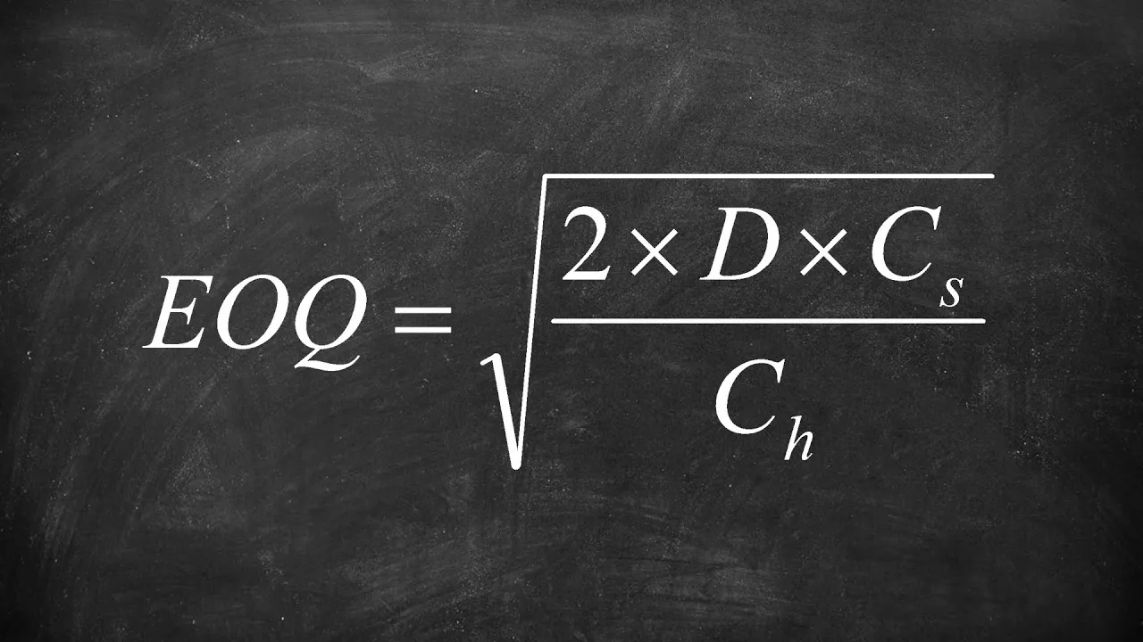
The next slide asks how to calculate EOQ and displays the formula EOQ=C×P2×(F×S). The speaker reads it aloud and treats it as the practical computation rule.
The symbol legend is then unpacked. F is the fixed cost of placing and receiving an order. S is annual sales in units. The speaker especially warns that the time basis matters: S must be annual, not weekly or another period used carelessly.
The denominator begins with C, defined on screen as carrying costs expressed as a percentage of inventory value, and P, the purchase price per unit. Below the main formula, the slide also lists two auxiliary expressions: total carrying costs =2Q×CC and total restocking costs =QF×T.
The segment opens on a static green slide titled “How do we calculate EOQ?” The main formula shown is EOQ=C×P2×(F×S). Beneath it, the legend defines EOQ as the economic order quantity, F as the fixed cost of placing and receiving an order, S as annual sales in units, C as carrying costs expressed as a percentage of inventory value, and P as purchase price per unit.
The speaker clarifies the meaning of C: it is not entered as an absolute cost, but as a ratio obtained by dividing carrying cost by inventory value. This matters because the denominator of the EOQ formula uses the percentage form of carrying cost together with the unit purchase price P.
The lecture then shifts from definition to data preparation. The speaker notes that some inputs may not appear in the exact form required by the formula. In particular, if only weekly sales are given, annual sales can be obtained by multiplying weekly sales by 52 weeks. Likewise, if the carrying-cost percentage is not stated directly, it must first be calculated.
Still on the same slide, the presenter introduces two auxiliary formulas used in EOQ examples. The first is total carrying costs, written as Total carrying costs=Average inventory×carrying costs per unit=2Q×CC. Here Q is described as the quantity in stock at a specific period, such as weekly or biweekly, and CC is carrying cost per unit.
The second auxiliary formula is total restocking costs: Total restocking costs=Fixed cost per order×number of orders=QF×T. The speaker identifies T as the annual quantity in units and explains that dividing T by the period quantity Q yields the number of orders. This connects the symbolic formula to the verbal idea of fixed cost per order multiplied by order frequency.
The slide changes to “Example 1,” introducing a word problem for Jersey Limited, a manufacturer of milk bottles. The visible data are: annual sales 500000 units, purchase price per unit R3, carrying cost equal to 20% of purchase price, ordering cost R100 per order, delivery time 4 days, and desired safety stock 4000 units.
Within this clip, the example is only set up and read aloud; no substitution into the EOQ formula is performed and no numerical answer is shown. The mathematical content therefore ends at the stage of identifying the given quantities that correspond to the variables introduced earlier.
The clip opens on a worked business-mathematics example titled Example 1. The visible problem states that Jersey Limited manufactures milk bottles and provides five data items: annual sales of 500 000 units, purchase price of R3 per unit, carrying cost equal to 20% of the purchase price of goods, ordering cost of R100 per order, delivery time of four days, and desired safety stock of 4 000 units. The lecturer reads these facts aloud, emphasizing the safety stock as important for the broader question.
A Required box then appears below the problem. It asks for two outputs: first, calculate the economic order quantity (EOQ) for Jersey Limited; second, determine the reorder point assuming a 360-day year. In this segment, only the first task is actually solved. The reorder-point inputs remain on screen but are not used yet.
The lecturer shifts to method by recalling the EOQ formula shown at the bottom left: EOQ=C×P2×F×S. The legend defines EOQ as the optimum order quantity per order, F as the fixed cost of placing and receiving an order, S as annual sales in units, C as carrying cost expressed as a percentage of inventory value, and P as purchase price per unit. This establishes the symbolic structure before any numbers are inserted.
The worked solution begins by matching each word-problem quantity to the formula symbols. The ordering cost R100 per order is assigned to F, so the numerator starts as 2×100. The lecturer then identifies S as annual demand in units and substitutes 500 000. While doing so, he adds a caution that if a question gives weekly sales, one must multiply by 52, and if it gives monthly sales, one must multiply by 12, because the formula requires annual units.
Next, the denominator is built. The carrying cost percentage 20% is entered as C=0.2, and the purchase price per unit is P=3. The lecturer explicitly treats C as a percentage of inventory value rather than as a currency amount, and the screen shows the full substituted expression EOQ=0.2×32×100×500000.
The expression is then evaluated numerically. The lecturer says to plug the formula into a calculator and reports 12909.95. He immediately reminds the viewer that EOQ is measured in units, so the answer should be rounded to a whole number. The slide shows the rounded result as approximately 12910 units.
The final part of the clip interprets the result rather than introducing new algebra. The lecturer explains that 12 910 is the order quantity corresponding to the optimal inventory level. He begins to contrast this with holding more or less than that amount, saying that quantities above 12 910 raise holding cost, while quantities below it affect the other cost side; the sentence is cut off before the explanation is completed.
The segment begins with the tail end of the EOQ calculation. On screen, the general formula EOQ=C×P2×(F×S) is still visible together with the worked substitution EOQ=0.2×32×100×500000, and the result is shown as 12909.95≈12910. The lecturer uses this to close part 2.1 and announce that part 2.2 asks for the reorder point under a 360-day year.
The lower EOQ boxes disappear, leaving the main problem statement and the Required section. A new yellow line appears: Re-order levels in units=Safety stock+Re-order point. The lecturer explains that safety stock is already given as 4 000 units, so the unknown piece is the reorder point itself.
A second yellow line is added: Reorder point=Waiting time×Daily average usage. The lecturer identifies the waiting time from the problem statement as 4 days, matching the sentence that four days are required for delivery.
To obtain daily average usage, the slide adds Daily average usage=500000/360=1388.89=1389. The lecturer explicitly notes that the divisor follows the problem’s instruction to assume a 360-day year, and mentions that some questions may instead use 365. The decimal result is then rounded to the nearest whole unit, 1389.
With both factors now known, the final yellow line appears: Reorder point=4×1389=5556. The lecturer states the conclusion directly: the reorder point for Jersey Limited is 5 556 units.
The video presents a static slide detailing an inventory management problem for Jersey Limited. The speaker begins by explaining the concept of re-order levels in units, emphasizing the need to include safety stock. The formula shown on the slide is Re-order levels in units = Safety stock + Re-order point.
The speaker then walks through the calculation of the daily average usage, which is derived by dividing the annual sales of 500,000 units by 360 days, resulting in approximately 1,389 units per day.
Next, the reorder point is calculated by multiplying the delivery time of 4 days by the daily average usage of 1,389 units, yielding a reorder point of 5,556 units.
Finally, the speaker calculates the total re-order levels in units by adding the desired safety stock of 4,000 units to the reorder point of 5,556 units, resulting in a total order quantity of 9,556 units.
The segment concludes with the speaker summarizing the process and encouraging viewers to ask questions or subscribe to the channel.
Knowledge cards
01
What EOQ is
EOQ is introduced as an inventory-management model used to establish optimal inventory levels. The video defines it as the optimum order quantity a company should hold given production cost, demand rate, and other variables, with the purpose of minimizing variable inventory costs.
02
Graphical meaning of EOQ
In the graph, the vertical axis is cost and the horizontal axis is order quantity. The holding-cost line rises with order quantity, the ordering-cost line falls, and EOQ is marked at their intersection. A U-shaped total-cost curve is drawn above them to show overall cost behavior.
03
Why holding and ordering costs move oppositely
The speaker explains that holding more inventory means ordering more at one time, and larger orders reduce ordering cost. Thus, as order quantity increases, holding cost goes up while ordering cost goes down, creating the tradeoff visualized in the graph.
04
EOQ formula
The calculation slide gives the standard formula shown on screen: EOQ equals the square root of two times F times S divided by C times P. The speaker presents this as the direct way to compute EOQ in questions.
EOQ=C×P2×(F×S)
05
Meaning of the symbols F, S, C, and P
F is the fixed cost of placing and receiving an order. S is annual sales in units. C is carrying costs expressed as a percentage of inventory value. P is the purchase price per unit. The speaker particularly stresses that S must be annual.
06
Auxiliary cost formulas on the same slide
Below the main EOQ formula, the slide adds two supporting expressions: total carrying costs equal average inventory times carrying costs per unit, written as Q x CC / 2, and total restocking costs equal fixed cost per order times number of orders, written as FxT/Q. These are shown visually but not verbally expanded in the clip.
Total carrying costs=2Q×CC,Total restocking costs=QF×T
07
EOQ formula
The video defines the Economic Order Quantity as the optimum order quantity per order and displays the formula EOQ=C×P2×(F×S). The legend assigns F to fixed ordering cost, S to annual sales in units, C to carrying cost as a percentage of inventory value, and P to purchase price per unit.
EOQ=C×P2×(F×S)
08
Meaning of C in EOQ
The speaker stresses that C must be expressed as a percentage of inventory value. To obtain it, divide carrying cost by inventory value. This distinguishes the rate C from an absolute carrying-cost amount.
C=inventory valuecarrying cost
09
Converting weekly sales to annual sales
Before using the EOQ formula, the problem data may need conversion. If weekly sales are given instead of annual sales, multiply by 52 weeks to obtain S in annual units.
Sannual=Sweekly×52
10
Total carrying costs formula
An auxiliary formula on the same slide computes total carrying costs as average inventory times carrying cost per unit, written 2Q×CC. The speaker explains Q as the quantity in stock at a specific period and CC as carrying cost per unit.
Total carrying costs=2Q×CC
11
Total restocking costs formula
The slide also gives total restocking costs as fixed cost per order times number of orders, written QF×T. The speaker identifies T as annual quantity in units and Q as the quantity at the relevant period, so T/Q represents the number of orders.
Total restocking costs=QF×T
12
Jersey Limited example data
Example 1 presents Jersey Limited with annual sales of 500 000 units, purchase price R3 per unit, carrying cost 20% of purchase price, ordering cost R100 per order, delivery time 4 days, and safety stock 4 000 units. The clip ends before any solution is calculated.
13
EOQ formula used in the example
The video presents the economic order quantity formula as EOQ=C×P2×F×S, where F is the fixed cost of placing and receiving an order, S is annual sales in units, C is carrying cost expressed as a percentage of inventory value, and P is purchase price per unit. The on-screen legend also describes EOQ as the optimum order quantity per order.
EOQ=C×P2×F×S
14
Mapping Jersey Limited data to the EOQ symbols
For the worked example, the lecturer assigns the given values as F=100, S=500000, C=0.2, and P=3. This produces the substituted expression EOQ=0.2×32×100×500000.
EOQ=0.2×32×100×500000
15
Annualize demand before using EOQ
The lecturer warns that the formula requires annual sales in units. If a problem gives weekly sales, multiply by 52; if it gives monthly sales, multiply by 12. In this example, annual sales are already given directly as 500 000 units.
16
Carrying cost is a percentage, not a currency amount
In this example, the carrying cost is 20% of the purchase price of goods, so the lecturer substitutes C=0.2 and multiplies it by P=3 in the denominator. This distinguishes the percentage rate C from a rand amount.
C=0.2,P=3
17
EOQ result and rounding
Evaluating the substituted expression gives 12909.95. Because EOQ is measured in units, the lecturer rounds the answer to 12910 units.
EOQ=12909.95≈12910
18
Business meaning of the EOQ answer
The clip interprets 12910 units as the order quantity that gives the optimal inventory level. The lecturer begins to explain that holding more than this increases holding cost, while holding less moves away from the optimum on the other cost side, but the sentence is cut off before completion.
19
Reorder point is requested but not solved in this clip
Although the Required section asks to determine the reorder point for Jersey Limited assuming a 360-day year, and the problem supplies delivery time of 4 days and safety stock of 4 000 units, this segment only solves the EOQ part. No reorder-point formula or calculation appears before the clip ends.
20
EOQ formula used in the example
The video presents the economic order quantity as EOQ=C×P2×(F×S), where F is the fixed cost per order, S is annual demand in units, C is the carrying-cost rate as a decimal, and P is the purchase price per unit. For Jersey Limited, the slide substitutes F=100, S=500000, C=0.2, and P=3, giving EOQ≈12910 units.
EOQ=C×P2×(F×S)
21
Reorder level definition
The reorder level in units is defined on screen as Re-order levels in units=Safety stock+Re-order point. In this example, safety stock is already known to be 4 000 units, so the remaining task is to compute the reorder point.
Re-order levels in units=Safety stock+Re-order point
22
Reorder point formula
The reorder point is calculated as Reorder point=Waiting time×Daily average usage. The waiting time is the delivery lead time, here 4 days, and the daily average usage must first be derived from annual demand.
Reorder point=Waiting time×Daily average usage
23
Daily average usage from annual demand
Daily average usage is obtained by dividing annual demand by the assumed number of days in the year. The slide computes Daily average usage=500000/360=1388.89≈1389 units per day, using the problem’s explicit 360-day-year assumption rather than 365 days.
Daily average usage=360500000=1388.89≈1389
24
Final reorder point for Jersey Limited
After rounding daily usage to 1389 units, the video multiplies by the 4-day waiting time: Reorder point=4×1389=5556 units. This is the final numerical answer shown for part 2.2 in the clip.
Reorder point=4×1389=5556
Detailed learning notes
Explore conditions, steps and evidence. Supplementary explanations are labeled separately from content shown in the video.
Symbols · 46
EOQ
Clear evidence
Shown in the video
Evidence
Caption evidence
Observation
Title slide shows "Economic Order Quantity (EOQ)".
Formula
Observation
Formula slide defines "EOQ = the economic order quantity (optimum order quantity per order)".
Audio
Observation
Speaker introduces the lesson as "the economic order quantity or the EOQ" and later says EOQ is calculated by the displayed formula.
Symbol
EOQ
Meaning
economic order quantity; optimum order quantity per order used to manage inventory and minimize variable inventory costs
Domain
order quantity per order
F
Clear evidence
Shown in the video
Evidence
Formula
Observation
Formula slide lists "F = fixed costs of placing and receiving an order".
Audio
Observation
Speaker says "F stands for the fixed costs of placing and receiving an order".
Symbol
F
Meaning
fixed costs of placing and receiving an order
Domain
cost per order
S
Clear evidence
Shown in the video
Evidence
Formula
Observation
Formula slide lists "S = the annual sales in units".
Audio
Observation
Speaker says "S stands for the annual sales in units" and emphasizes using annual rather than weekly figures.
Symbol
S
Meaning
annual sales in units
Domain
units per year
C
Clear evidence
Shown in the video
Evidence
Formula
Observation
Formula slide lists "C = the carrying costs expressed as a percentage of inventory value".
Audio
Observation
Speaker begins defining C as "the carrying costs expressed as a percentage" before the clip ends.
Uncertainties
The spoken definition of C is cut off before completion, but the on-screen text fully states it.
Symbol
C
Meaning
carrying costs expressed as a percentage of inventory value
Domain
percentage of inventory value
P
Clear evidence
Shown in the video
Evidence
Formula
Observation
Formula slide lists "P = the purchase price per unit".
Uncertainties
The speaker does not reach P verbally within this clip.
Symbol
P
Meaning
purchase price per unit
Domain
price per unit
Q
Clear evidence
Shown in the video
Evidence
Formula
Observation
Auxiliary formulas show "Total carrying costs = Average inventory x carrying costs per unit = Q x CC / 2" and "Total restocking costs = Fixed cost per order x number of orders = FxT/Q".
Uncertainties
The slide does not explicitly define Q or T in the visible text.
Symbol
Q
Meaning
quantity variable appearing in auxiliary carrying-cost and restocking-cost formulas
Domain
not explicitly defined on screen
CC
Clear evidence
Shown in the video
Evidence
Formula
Observation
Auxiliary formula uses "CC" in "Q x CC / 2" under "Total carrying costs".
Uncertainties
The slide does not explicitly define CC in the visible text.
Symbol
CC
Meaning
carrying costs per unit in the auxiliary total carrying cost formula
Domain
not explicitly defined on screen
T
Clear evidence
Shown in the video
Evidence
Formula
Observation
Auxiliary formula uses "T" in "FxT/Q" under "Total restocking costs".
Uncertainties
The slide does not explicitly define T in the visible text.
Symbol
T
Meaning
variable in the auxiliary total restocking cost formula
Domain
not explicitly defined on screen
$
Clear evidence
Shown in the video
Evidence
Diagram
Observation
Graph vertical axis is labeled "Costs" with "$".
Symbol
$
Meaning
monetary cost scale on the vertical axis of the EOQ graph
Domain
cost
EOQ
Clear evidence
Shown in the video
Evidence
Formula
Observation
Slide text defines EOQ = the economic order quantity (optimum order quantity per order).
Audio
Observation
Speaker refers to the EOQ formula and says this is how you go ahead with the EOQ formula.
Symbol
EOQ
Meaning
economic order quantity; optimum order quantity per order
Domain
order quantity in units
F
Clear evidence
Shown in the video
Evidence
Formula
Observation
Slide text defines F = fixed costs of placing and receiving an order.
Audio
Observation
Speaker says F, which is the fixed cost per order.
Symbol
F
Meaning
fixed cost of placing and receiving one order
Domain
cost per order
S
Clear evidence
Shown in the video
Evidence
Formula
Observation
Slide text defines S = the annual sales in units.
Audio
Observation
Speaker says annual sales in units may need to be calculated from weekly sales by multiplying by 52 weeks.
Symbol
S
Meaning
annual sales in units
Domain
units per year
Knowledge points · 19
Definition and purpose of EOQ
Clear evidence
Shown in the video
Evidence
Caption evidence
Observation
Slide text: "It is a model commonly used to establish optimal inventory levels. It is used to manage inventory".
Caption evidence
Observation
Slide text: "In other words, it is the optimum order quantity that a company should hold in its inventory given a set cost of production, demand rate and other variables. This is done to minimize variable inventory costs."
Audio
Observation
Speaker says EOQ is a model used to establish optimal inventory levels and manage inventory.
Audio
Observation
Speaker says EOQ is the optimum order quantity a company should hold given production cost, demand rate, and other variables, and that it is done to minimize variable inventory costs.
Definition
Explanation
EOQ is presented as an inventory-management model whose purpose is to determine the optimum order quantity a company should hold so that variable inventory costs are minimized. The video frames EOQ as a tool for establishing optimal inventory levels rather than as a general accounting measure.
Formula
Conditions
Used to manage inventory
Given a set cost of production, demand rate, and other variables
Aimed at minimizing variable inventory costs
EOQ calculation formula
Clear evidence
Shown in the video
Evidence
Formula
Observation
Slide displays "EOQ = C×P2×(F×S)".
Audio
Observation
Speaker reads the formula as the square root of two times F times S divided by C times P.
Formula
Observation
Slide defines EOQ, F, S, C, and P in the legend beneath the formula.
Formula
Explanation
The clip gives the standard EOQ expression as the square root of twice the product of ordering cost and annual sales divided by the product of carrying-cost percentage and purchase price per unit. The speaker emphasizes that this formula is the practical way to compute EOQ in questions.
Formula
EOQ=C×P2×(F×S)
Conditions
F is fixed cost of placing and receiving an order
S is annual sales in units
C is carrying cost expressed as a percentage of inventory value
P is purchase price per unit
Prerequisites
Definition and purpose of EOQ
Meanings of EOQ formula symbols
Clear evidence
Shown in the video
Evidence
Formula
Observation
Legend on slide: "EOQ = the economic order quantity (optimum order quantity per order)".
Formula
Observation
Legend on slide: "F = fixed costs of placing and receiving an order".
Formula
Observation
Legend on slide: "S = the annual sales in units".
Formula
Observation
Legend on slide: "C = the carrying costs expressed as a percentage of inventory value".
Formula
Observation
Legend on slide: "P = the purchase price per unit".
Audio
Observation
Speaker explains F, S, and begins explaining C while pointing around the formula legend.
Uncertainties
The spoken explanation reaches only partway through C before the clip ends.
Definition
Explanation
The formula slide assigns each symbol a specific inventory-cost role: EOQ is the optimum order quantity per order, F is the fixed cost of placing and receiving an order, S is annual sales in units, C is carrying cost as a percentage of inventory value, and P is purchase price per unit. The speaker especially stresses that S must be annual rather than weekly.
Formula
Conditions
Symbols are used together in the EOQ formula
S must be measured on an annual basis
Prerequisites
EOQ calculation formula
Auxiliary carrying-cost and restocking-cost formulas
Clear evidence
Shown in the video
Evidence
Formula
Observation
Slide text: "Two other formulae provide useful analyses:".
Formula
Observation
Slide text: "Total carrying costs = Average inventory x carrying costs per unit = Q x CC / 2".
Formula
Observation
Slide text: "Total restocking costs = Fixed cost per order x number of orders = FxT/Q".
Uncertainties
Q, CC, and T are shown without explicit definitions on the slide.
These auxiliary formulas are visible but not verbally explained within the clip.
Formula
Explanation
Below the main EOQ formula, the slide adds two supporting expressions for analysis: total carrying costs equal average inventory times carrying cost per unit, written as Q x CC / 2, and total restocking costs equal fixed cost per order times number of orders, written as FxT/Q. These formulas connect the EOQ idea to separate cost components.
Formula
Total carrying costs=2Q×CC,Total restocking costs=QF×T
Conditions
Presented as useful analyses alongside the EOQ formula
Variables Q, CC, and T are not explicitly defined on screen
Prerequisites
EOQ calculation formula
EOQ formula
Clear evidence
Shown in the video
Evidence
Formula
Observation
Slide displays EOQ = sqrt((2x(FxS))/(C x P)).
Formula
Observation
Slide legend defines EOQ, F, S, C, and P.
Audio
Observation
Speaker explains C as a percentage of inventory value and P as purchase price per unit, then summarizes this as the EOQ formula.
Formula
Explanation
The video presents the Economic Order Quantity as the optimum order quantity per order. The formula shown is EOQ = sqrt((2x(FxS))/(C x P)), where F is the fixed cost of placing and receiving an order, S is annual sales in units, C is carrying cost expressed as a percentage of inventory value, and P is purchase price per unit.
Formula
EOQ=C×P2×(F×S)
Conditions
F is the fixed cost per order.
S is annual sales in units.
C is carrying cost as a percentage of inventory value.
P is purchase price per unit.
Carrying cost expressed as a percentage
Clear evidence
Shown in the video
Evidence
Formula
Observation
Slide legend states C = the carrying costs expressed as a percentage of inventory value.
Audio
Observation
Speaker says you take the carrying cost divided by the inventory value to get that percentage.
Definition
Explanation
The variable C is not an absolute cost amount in the EOQ formula; it is the carrying cost rate expressed as a percentage of inventory value. The speaker describes obtaining it by dividing carrying cost by inventory value.
Formula
C=inventory valuecarrying cost
Conditions
The result is used as a percentage in the EOQ denominator.
Inventory value must correspond to the same basis as the carrying cost.
Prerequisites
EOQ formula
Preparing inputs for EOQ
Clear evidence
Shown in the video
Evidence
Audio
Observation
Speaker says annual sales in units may not be given directly; weekly sales may be given and multiplied by 52 weeks to get annual sales.
Audio
Observation
Speaker also says the percentage may need to be calculated if not given.
Method
Explanation
Before applying the EOQ formula, some inputs may need conversion. If only weekly sales are given, the speaker says to multiply by 52 weeks to obtain annual sales. If the carrying-cost percentage is not given directly, it must be calculated first.
Formula
Sannual=Sweekly×52
Conditions
Use when the problem gives weekly sales instead of annual sales.
Use when C is not already expressed as a percentage of inventory value.
Prerequisites
EOQ formula
Carrying cost expressed as a percentage
Total carrying costs formula
Clear evidence
Shown in the video
Evidence
Formula
Observation
Slide displays Total carrying costs = Average inventory x carrying costs per unit = (Q x CC)/2.
Audio
Observation
Speaker says Q is the quantity in stock at a specific period, divide by two, then multiply by carrying costs per unit.
Formula
Explanation
The video gives an auxiliary formula for total carrying costs. It is computed as average inventory multiplied by carrying costs per unit, written on the slide as (Q x CC)/2. The speaker interprets Q as the quantity held in stock during the relevant period.
Formula
Total carrying costs=Average inventory×carrying costs per unit=2Q×CC
Conditions
Q is the quantity in stock at the specified period.
CC is carrying costs per unit.
The formula assumes average inventory is Q/2.
Total restocking costs formula
Clear evidence
Shown in the video
Evidence
Formula
Observation
Slide displays Total restocking costs = Fixed cost per order x number of orders = (F x T)/Q.
Audio
Observation
Speaker says take F, multiply by the total annual quantity, then divide by the quantity at the given period.
Formula
Explanation
The video gives an auxiliary formula for total restocking costs. It is computed as fixed cost per order multiplied by the number of orders, written on the slide as (F x T)/Q. The speaker identifies T as the annual quantity in units and Q as the quantity at the given period.
Formula
Total restocking costs=Fixed cost per order×number of orders=QF×T
Conditions
F is fixed cost per order.
T is annual quantity in units.
Q is the quantity at the specified ordering period.
T/Q represents the number of orders.
Economic order quantity formula
Clear evidence
Shown in the video
Evidence
Formula
Observation
Bottom-left box displays EOQ = sqrt((2 x F x S)/(C x P)) with a legend defining each variable.
Audio
Observation
The lecturer says, 'let's remind ourselves of the formula' and reads it as square root of two times F times S divided by C times P.
Formula
Explanation
The video presents the EOQ formula as the square root of the product of 2, the fixed ordering cost, and annual sales units, divided by the product of the carrying-cost percentage and the purchase price per unit. The on-screen legend explicitly defines EOQ as the optimum order quantity per order.
Formula
EOQ=C×P2×F×S
Conditions
F is the fixed cost of placing and receiving an order
S is annual sales in units
C is carrying cost expressed as a percentage of inventory value
P is purchase price per unit
EOQ is measured in units
Convert non-annual demand to annual units before using EOQ
Clear evidence
Shown in the video
Evidence
Audio
Observation
The lecturer says that if weekly sales are given, multiply by 52, and if monthly sales are given, multiply by 12.
Caption evidence
Observation
The problem itself gives annual sales directly as 500 000 units.
Method
Explanation
Before substituting into the EOQ formula, demand must be expressed as annual sales in units. The lecturer explicitly notes that weekly sales should be multiplied by 52 and monthly sales by 12 when the problem does not already provide annual figures.
Formula
Conditions
Use only when the given demand is not already annual
Weekly demand is converted by multiplying by 52
Monthly demand is converted by multiplying by 12
Prerequisites
Economic order quantity formula
Interpretation of EOQ as optimal stock level
Clear evidence
Shown in the video
Evidence
Audio
Observation
The lecturer says the EOQ is the actual unit that we need to have in stock to have the optimal inventory level.
Audio
Observation
He adds that anything over 12 910 raises holding cost, while anything less affects the other cost side.
Uncertainties
The lecturer begins to explain the cost consequence of ordering less than EOQ, but the sentence is cut off before he completes the thought.
Definition
Explanation
The video interprets the computed EOQ as the order size that gives the optimal inventory level. Quantities above this level increase holding cost, and quantities below it move away from the optimum on the other cost side.
Formula
Conditions
Applies to the EOQ result after substitution and rounding
Describes the business meaning of the computed quantity
Prerequisites
Economic order quantity formula
Claims and conditions · 4
EOQ is located at the intersection of holding cost and ordering cost
Clear evidence
Shown in the video
Evidence
Caption evidence
Observation
Slide text: "Notice how as the cost of holding goes up, the cost of ordering goes down. The EOQ is where they intersect."
Audio
Observation
Speaker says that when holding cost goes up, ordering cost goes down, and that EOQ lies where the two lines intersect.
Diagram
Observation
Graph labels one rising line "Cost of Holding", one falling line "Cost of Ordering", and marks the intersection with a dashed vertical line labeled "EOQ".
Proposition
Statement
In the graphical representation, EOQ is the order quantity at which the cost of holding and the cost of ordering intersect.
Hypotheses
The graph is interpreted as showing holding cost increasing with order quantity and ordering cost decreasing with order quantity.
Quantifiers
For the order quantity shown on the horizontal axis, the EOQ point is the intersection of the two plotted cost curves.
Holding cost and ordering cost move in opposite directions with order quantity
Clear evidence
Shown in the video
Evidence
Caption evidence
Observation
Slide text states that as holding cost goes up, ordering cost goes down.
Audio
Observation
Speaker explains that holding more inventory means ordering more, and the more inventory ordered, the less the cost of ordering becomes.
Diagram
Observation
The graph shows an upward-sloping holding-cost line and a downward-sloping ordering-cost line.
Proposition
Statement
As order quantity increases in the depicted model, holding cost rises while ordering cost falls.
Hypotheses
Order quantity is the horizontal-axis variable in the graph.
The plotted lines represent holding cost and ordering cost respectively.
Quantifiers
Across the displayed range of order quantity, the two cost trends are oppositely directed.
The demand term S must use annual units
Clear evidence
Shown in the video
Evidence
Audio
Observation
Speaker says it is important when calculating EOQ to bear in mind when you are using annual and when you are using weekly or whatever the case may be.
Audio
Observation
Speaker repeats that S stands for the annual sales in units.
Formula
Observation
Slide legend defines S as "the annual sales in units".
Proposition
Statement
In the EOQ formula shown, S represents annual sales in units, so the time basis must be annual rather than weekly or another period.
Hypotheses
The formula is being applied as written on the slide.
Quantifiers
For use of the displayed EOQ formula, the S input is annual sales in units.
EOQ result is expressed in units
Clear evidence
Shown in the video
Evidence
Audio
Observation
The lecturer says, 'remember the economic order quantity is in units. The answer will be in units.'
Proposition
Statement
The economic order quantity calculated by the displayed formula is measured in units.
Hypotheses
The variables are substituted according to the on-screen definitions
S is annual sales in units
P is price per unit
C is a percentage of inventory value
Quantifiers
for the EOQ calculation shown in this example
Derivations and proofs · 10
Graphical intuition for why EOQ is at the intersection
Clear evidence
Shown in the video
Evidence
Diagram
Observation
Graph shows axes "Costs ($)" and "Order Qty", with a rising "Cost of Holding" line, a falling "Cost of Ordering" line, and a U-shaped "Total Cost" curve above them.
Audio
Observation
Speaker explains that holding more inventory means ordering more, and the more inventory ordered, the less the cost of ordering becomes.
Caption evidence
Observation
Text says the EOQ is where holding cost and ordering cost intersect.
Uncertainties
The video gives a qualitative graphical explanation only; no algebraic derivation is shown in this clip.
Intuitive argument
Steps
Expression
Explanation
The graph uses order quantity on the horizontal axis and cost on the vertical axis.
Justification
Directly read from the axis labels "Order Qty" and "Costs ($)".
Shown in the video
Expression
Explanation
One plotted line rises with order quantity and is labeled "Cost of Holding".
Justification
Visible label and upward slope on the graph.
Shown in the video
Expression
Explanation
Another plotted line falls with order quantity and is labeled "Cost of Ordering".
Justification
Visible label and downward slope on the graph.
Shown in the video
Expression
Explanation
The speaker interprets the falling ordering-cost line as arising because larger orders mean fewer ordering events, reducing ordering cost.
Justification
Audio explanation: holding more inventory means ordering more, and the more inventory ordered, the less the cost of ordering becomes.
Shown in the video
Expression
Explanation
The intersection of the holding-cost and ordering-cost lines is marked by a dashed vertical line labeled "EOQ".
Justification
Visible graph annotation and matching slide text.
Shown in the video
Expression
Explanation
A U-shaped "Total Cost" curve is drawn above the two component lines, visually indicating that total cost is minimized near the same order quantity region.
Justification
Visible graph label "Total Cost" and curve shape; the video does not verbally derive the curve equation.
Shown in the video
Conclusion
The clip explains EOQ intuitively as the order quantity where opposing holding and ordering cost trends balance, with total cost shown as a U-shaped curve above them.
Reading the EOQ formula from the slide
Clear evidence
Shown in the video
Evidence
Formula
Observation
Slide displays the EOQ formula and a symbol legend.
Audio
Observation
Speaker reads the formula and then identifies F, S, and begins identifying C.
Uncertainties
No algebraic proof of the formula is provided in the clip.
Visual argument
Steps
Expression
EOQ=C×P2×(F×S)
Explanation
The main formula is presented directly on the slide.
Justification
Visible formula text.
Shown in the video
Expression
F=fixed costs of placing and receiving an order
Explanation
The numerator contains F as the ordering-related fixed cost.
Justification
Slide legend and speaker's verbal identification of F.
Shown in the video
Expression
S=annual sales in units
Explanation
The numerator also contains S as annual demand measured in units.
Justification
Slide legend and speaker's emphasis on annual rather than weekly usage.
Shown in the video
Expression
C=carrying costs expressed as a percentage of inventory value
Explanation
The denominator contains C as the carrying-cost percentage.
Justification
Slide legend; speaker begins this definition before the clip ends.
Shown in the video
Expression
P=purchase price per unit
Explanation
The denominator also contains P as unit purchase price.
Justification
Visible slide legend.
Shown in the video
Conclusion
The formula combines ordering cost and annual demand in the numerator, and carrying-cost percentage times unit price in the denominator, under a square root.
Preparing variables before substituting into EOQ
Clear evidence
Shown in the video
Evidence
Audio
Observation
Speaker explains how C is obtained as a percentage and how annual sales may be derived from weekly sales.
Formula
Observation
Slide legend defines C and S for use in the EOQ formula.
Intuitive argument
Steps
Expression
C=inventory valuecarrying cost
Explanation
Convert carrying cost into the percentage form required by the EOQ formula.
Justification
The slide defines C as carrying costs expressed as a percentage of inventory value, and the speaker says to divide carrying cost by inventory value.
Shown in the video
Expression
Sannual=Sweekly×52
Explanation
If only weekly sales are supplied, convert them to annual sales before substitution.
Justification
The speaker explicitly says weekly sales may need to be multiplied by 52 weeks to get annual sales.
Shown in the video
Expression
EOQ=C×P2×(F×S)
Explanation
Substitute the prepared values of F, S, C, and P into the displayed EOQ formula.
Justification
This is the formula shown on the slide after the variable definitions.
Shown in the video
Conclusion
The EOQ calculation requires F, annual S, percentage C, and unit price P; if any of these are not directly given, they must first be converted or calculated.
Substitution and evaluation of EOQ for Jersey Limited
Clear evidence
Shown in the video
Evidence
Formula
Observation
The right-hand calculation box builds step by step from EOQ = sqrt(2 x ... ) to EOQ = sqrt((2 x 100 x 500 000)/(0.2 x 3)).
Audio
Observation
The lecturer substitutes F=100, S=500000, C=0.2, and P=3, then states the calculator result 12 909.95 and rounds to 12 910.
Numerical verification
Steps
Expression
EOQ=C×P2×F×S
Explanation
Start from the general EOQ formula shown at the bottom left.
Justification
On-screen formula and spoken reminder of the formula.
Shown in the video
Expression
F=100
Explanation
Identify the fixed ordering cost from the problem statement.
Justification
The problem text says the ordering cost is R100 per order, and the lecturer maps this to F.
Shown in the video
Expression
S=500000
Explanation
Identify annual sales in units from the problem statement.
Justification
The problem text says annual sales amount to 500 000 units, and the lecturer maps this to S.
Shown in the video
Expression
C=0.2
Explanation
Convert the carrying cost percentage into decimal form.
Justification
The problem states carrying cost is 20% of purchase price of goods; the lecturer substitutes 0.2 for C.
Shown in the video
Expression
P=3
Explanation
Identify the purchase price per unit.
Justification
The problem text states the purchasing price per unit is R3, and the lecturer maps this to P.
Shown in the video
Expression
EOQ=0.2×32×100×500000
Explanation
Substitute all identified values into the formula.
Justification
Direct substitution into the displayed EOQ formula.
Shown in the video
Expression
EOQ=12909.95
Explanation
Evaluate the expression numerically.
Justification
The lecturer says to plug it into a calculator and reports 12 909.95.
Shown in the video
Expression
EOQ≈12910
Explanation
Round the numerical result to the nearest whole unit.
Justification
The lecturer says to round up to the nearest number and the screen shows approximately 12 910.
Shown in the video
Conclusion
For Jersey Limited, the economic order quantity is approximately 12 910 units.
Independent check of the EOQ arithmetic
Clear evidence
Supplementary explanation
Evidence
Formula
Observation
Using the same substituted expression from the video allows independent arithmetic verification.
Numerical verification
Steps
Expression
0.2×32×100×500000=0.6100000000
Explanation
Multiply the numerator and denominator separately.
Justification
Standard arithmetic simplification of the substituted formula.
Supplementary explanation
Expression
0.6100000000=166666666.666…
Explanation
Divide to obtain the value inside the square root.
Justification
Arithmetic evaluation.
Supplementary explanation
Expression
166666666.666…≈12909.9445
Explanation
Take the square root to recover EOQ.
Justification
Definition of the EOQ formula after substitution.
Supplementary explanation
Expression
12909.9445≈12910
Explanation
Round to the nearest whole unit.
Justification
Rounding convention stated by the lecturer.
Supplementary explanation
Conclusion
The independently checked value agrees with the video's rounded EOQ of 12 910 units.
EOQ numerical evaluation from the displayed substitution
Clear evidence
Shown in the video
Evidence
Formula
Observation
The worked expression on screen substitutes the given values into the EOQ formula: EOQ = sqrt((2 X 100 X 500 000)/(0,2 X 3)).
Formula
Observation
The right side of the slide shows 12 909,95 and then ≈ 12 910.
Audio
Observation
The lecturer says the optimal inventory level has just been calculated as 12 910.
Numerical verification
Steps
Expression
EOQ=0.2×32×100×500000
Explanation
The video substitutes F=100, S=500000, C=0.2, and P=3 into the EOQ formula.
Justification
Direct substitution using the values shown in the problem statement and formula legend.
Shown in the video
Expression
=12909.95≈12910
Explanation
The slide reports the evaluated EOQ as 12 909,95 and rounds it to 12 910.
Justification
Displayed numerical result and rounding on the slide.
Shown in the video
Conclusion
The economic order quantity for Jersey Limited is approximately 12 910 units.
Derivation of the reorder point from annual demand and lead time
Clear evidence
Shown in the video
Evidence
Formula
Observation
The slide first shows Re-order levels in units = Safety stock + Re-order point.
Formula
Observation
It then shows Reorder point = Waiting time X Daily average usage.
Formula
Observation
Next it shows Daily average usage = 500000/360=1388.89=1389.
Formula
Observation
Finally it shows Reorder point = 4X1389=5556.
Audio
Observation
The lecturer walks through these steps verbally in the same order.
Numerical verification
Steps
Expression
Re-order levels in units=Safety stock+Re-order point
Explanation
The lecturer starts from the definition of the reorder level and identifies safety stock as already known.
Justification
On-screen formula and spoken explanation.
Shown in the video
Expression
Reorder point=Waiting time×Daily average usage
Explanation
Because the reorder point is not yet known, the video introduces the formula needed to compute it.
Justification
On-screen formula and spoken explanation.
Shown in the video
Expression
Daily average usage=360500000=1388.89≈1389
Explanation
Annual demand is converted to a daily figure using the stated 360-day year, then rounded to the nearest whole unit.
Justification
Problem statement plus displayed arithmetic.
Shown in the video
Expression
Reorder point=4×1389=5556
Explanation
The waiting time of 4 days is multiplied by the rounded daily usage of 1389 units.
Justification
Displayed substitution and multiplication.
Shown in the video
Conclusion
The reorder point is 5 556 units.
Calculation of Daily Average Usage
Clear evidence
Shown in the video
Evidence
Diagram
Observation
Slide text shows 'Daily average usage = 500000/360=1388.89=1389'.
Numerical verification
Steps
Expression
500000/360
Explanation
Divide the annual sales amount by the number of days in a year (assuming a 360-day year).
Justification
To find the average daily usage.
Shown in the video
Expression
1388.89≈1389
Explanation
Round the result to the nearest whole number.
Justification
Units are typically counted as whole numbers.
Shown in the video
Conclusion
The daily average usage is 1,389 units.
Calculation of Reorder Point
Clear evidence
Shown in the video
Evidence
Diagram
Observation
Slide text shows 'Reorder point = 4X1389=5556'.
Numerical verification
Steps
Expression
4×1389
Explanation
Multiply the delivery time (waiting time) by the daily average usage.
Justification
To find the inventory level at which a new order should be placed.
Shown in the video
Expression
5556
Explanation
Calculate the product.
Justification
Arithmetic calculation.
Shown in the video
Conclusion
The reorder point is 5,556 units.
Calculation of Re-order Levels in Units
Clear evidence
Shown in the video
Evidence
Diagram
Observation
Slide text shows 'Reorder levels in units = 4000+5556=9556 units'.
Numerical verification
Steps
Expression
4000+5556
Explanation
Add the safety stock to the reorder point.
Justification
To find the total quantity to order each time.
Shown in the video
Expression
9556
Explanation
Calculate the sum.
Justification
Arithmetic calculation.
Shown in the video
Conclusion
The re-order levels in units is 9,556 units.
Worked examples · 4
Jersey Limited EOQ example setup
Clear evidence
Shown in the video
Evidence
Formula
Observation
Slide title changes to Example 1 and displays the problem statement for Jersey Limited.
Audio
Observation
Speaker reads the example setup: Jersey Limited is a manufacturer of milk bottles, annual sales 500,000 units, purchase price R3, carrying cost 20% of purchase price, ordering cost R100 per order, four days required for delivery.
Uncertainties
The clip ends before the solution is worked out; no EOQ numerical answer is shown or spoken within this segment.
Problem
2.1 Jersey Limited is a manufacturer of milk bottles. The following information is obtained from their records: Annual sales amount to 500 000 units. The purchasing price per unit is R3. The carrying cost of inventory is equal to 20% of the purchase price of goods. The ordering cost is R100 per order. Four days are required for delivery. The desired safety stock for the firm is 4 000 units.
Given
Annual sales = 500 000 units.
Purchase price per unit = R3.
Carrying cost of inventory = 20% of purchase price of goods.
Ordering cost = R100 per order.
Delivery time = 4 days.
Desired safety stock = 4 000 units.
Goal
Set up the data for an EOQ-related example; the explicit target question is not reached within this clip.
Steps
Expression
S=500000
Explanation
Record annual sales in units.
Justification
The slide states annual sales amount to 500 000 units.
Shown in the video
Expression
P=3
Explanation
Record purchase price per unit in rand.
Justification
The slide states the purchasing price per unit is R3.
Shown in the video
Expression
C=0.20
Explanation
Express the carrying cost as a decimal percentage of purchase price.
Justification
The slide states carrying cost is equal to 20% of the purchase price of goods.
Shown in the video
Expression
F=100
Explanation
Record fixed ordering cost per order.
Justification
The slide states the ordering cost is R100 per order.
Shown in the video
Expression
delivery time=4 days,safety stock=4000 units
Explanation
Record the additional operational data shown on the slide.
Justification
These values appear in the example statement but are not used before the clip ends.
Shown in the video
Answer
No final numerical answer is provided within this 150-second clip.
Verification
The extracted values match the visible Example 1 slide text exactly; the absence of a solution is confirmed by the clip ending immediately after the setup.
Jersey Limited EOQ example
Clear evidence
Shown in the video
Evidence
Caption evidence
Observation
Slide title reads Example 1 and the problem text describes Jersey Limited, a manufacturer of milk bottles, with annual sales 500 000 units, purchase price R3, carrying cost 20%, ordering cost R100 per order, delivery 4 days, and safety stock 4 000 units.
Caption evidence
Observation
Required section asks to calculate EOQ and determine the reorder point assuming a 360-day year.
Formula
Observation
The worked solution on the right computes EOQ = sqrt((2 x 100 x 500 000)/(0.2 x 3)) and shows 12 909.95, then approximately 12 910.
Uncertainties
The second required item, the reorder point, is stated in the problem but not solved within this clip.
Problem
Jersey Limited is a manufacturer of milk bottles. Annual sales amount to 500 000 units. The purchasing price per unit is R3. The carrying cost of inventory is equal to 20% of the purchase price of goods. The ordering cost is R100 per order. Four days are required for delivery. The desired safety stock for the firm is 4 000 units. Required: calculate the economic order quantity (EOQ) for Jersey Limited.
Given
Annual sales = 500 000 units
Purchase price per unit = R3
Carrying cost = 20% of purchase price of goods
Ordering cost = R100 per order
Delivery time = 4 days
Safety stock = 4 000 units
Assume a 360-day year for the reorder-point question
Goal
Compute the economic order quantity (EOQ) for Jersey Limited.
Steps
Expression
EOQ=C×P2×F×S
Explanation
Write the EOQ formula from the slide.
Justification
Given formula in the bottom-left box.
Shown in the video
Expression
F=100,S=500000,C=0.2,P=3
Explanation
Match each word-problem quantity to the corresponding symbol.
Justification
Definitions in the slide legend and the lecturer's spoken mapping.
Shown in the video
Expression
EOQ=0.2×32×100×500000
Explanation
Substitute the identified values into the formula.
Justification
Direct substitution.
Shown in the video
Expression
EOQ=12909.95
Explanation
Evaluate the expression numerically.
Justification
Calculator result stated by the lecturer and shown on screen.
Shown in the video
Expression
EOQ≈12910
Explanation
Round to the nearest whole unit.
Justification
The lecturer says to round up to the nearest number because EOQ is in units.
Shown in the video
Answer
EOQ ≈12910 units
Verification
Independent arithmetic gives sqrt(100000000/0.6) = 12909.9445..., which rounds to 12910, matching the video.
Jersey Limited EOQ and reorder point example
Clear evidence
Shown in the video
Evidence
Caption evidence
Observation
The slide states: Jersey Limited is a manufacturer of milk bottles. Annual sales amount to 500 000 units. The purchasing price per unit is R3. The carrying cost of inventory is equal to 20% of the purchase price of goods. The ordering cost is R100 per order. Four days are required for delivery. The desired safety stock for the firm is 4 000 units.
Caption evidence
Observation
The Required section asks to calculate the EOQ and determine the re-order point, assuming a 360-day year.
Formula
Observation
The worked EOQ line and the later reorder-point lines are shown on the same slide.
Problem
For Jersey Limited, calculate the economic order quantity and then determine the reorder point using the given inventory data and a 360-day year.
Given
Annual sales = 500 000 units
Purchase price per unit = R3
Carrying cost = 20% of purchase price
Ordering cost = R100 per order
Delivery waiting time = 4 days
Desired safety stock = 4 000 units
Assume a 360-day year
Goal
Compute EOQ and the reorder point in units.
Steps
Expression
EOQ=0.2×32×100×500000
Explanation
Substitute the given ordering cost, annual demand, carrying-cost rate, and unit price into the EOQ formula.
Justification
Direct application of the displayed EOQ formula.
Shown in the video
Expression
EOQ≈12910
Explanation
The slide evaluates the expression as 12 909,95 and rounds it to 12 910 units.
Justification
Displayed numerical result.
Shown in the video
Expression
Re-order levels in units=Safety stock+Re-order point
Explanation
To answer part 2.2, the lecturer first writes the relationship between reorder level, safety stock, and reorder point.
Justification
On-screen formula.
Shown in the video
Expression
Daily average usage=360500000=1388.89≈1389
Explanation
Convert annual demand to daily demand using the stated 360-day year and round to the nearest whole unit.
Justification
Problem assumption plus displayed arithmetic.
Shown in the video
Expression
Reorder point=4×1389=5556
Explanation
Multiply the 4-day waiting time by the rounded daily usage to obtain the reorder point.
Justification
Displayed substitution into the reorder-point formula.
Shown in the video
Answer
EOQ ≈ 12 910 units; Reorder point = 5 556 units.
Verification
The verification visible in the clip is the direct substitution of the stated data into the displayed formulas and the rounding shown on screen.
Jersey Limited Inventory Management Example
Clear evidence
Shown in the video
Evidence
Diagram
Observation
Slide presents the problem statement for Jersey Limited, including all given values and the required calculations.
Audio
Observation
Speaker walks through the calculations for the reorder point and re-order levels in units.
Problem
Jersey Limited is a manufacturer of milk bottles. Annual sales amount to 500,000 units. The purchasing price per unit is R3. The carrying cost of inventory is equal to 20% of the purchase price of goods. The ordering cost is R100 per order. Four days are required for delivery. The desired safety stock for the firm is 4,000 units. Determine the re-order point and re-order levels in units. Assume a 360-day year.
Given
Annual sales = 500,000 units
Purchasing price per unit = R3
Carrying cost = 20% of purchase price
Ordering cost = R100 per order
Delivery time = 4 days
Safety stock = 4,000 units
Days in a year = 360
Goal
Determine the re-order point and re-order levels in units.
Steps
Expression
Daily average usage=500000/360=1388.89≈1389
Explanation
Calculate the daily average usage by dividing annual sales by the number of days in a year.
Justification
Definition of daily average usage.
Shown in the video
Expression
Reorder point=4×1389=5556
Explanation
Calculate the reorder point by multiplying the delivery time by the daily average usage.
Justification
Definition of reorder point.
Shown in the video
Expression
Re-order levels in units=4000+5556=9556
Explanation
Calculate the re-order levels in units by adding the safety stock to the reorder point.
Justification
Definition of re-order levels in units.
Shown in the video
Answer
The re-order point is 5,556 units, and the re-order levels in units is 9,556 units.
Verification
The calculations follow the standard formulas for inventory management as presented in the video.
Visual events · 10
Title and definition slides for EOQ
Clear evidence
Shown in the video
Evidence
Caption evidence
Observation
Opening green title slide reads "Economic Order Quantity (EOQ)".
Caption evidence
Observation
Subsequent bullet slide adds the definition text about optimal inventory levels and minimizing variable inventory costs.
Audio
Observation
Speaker introduces the topic and reads/paraphrases the definition bullets.
Objects
Green background
Yellow title text "Economic Order Quantity (EOQ)"
White bullet text defining EOQ
Changes
The title remains while explanatory bullet text appears beneath it.
The second bullet expands the definition from inventory management to optimum order quantity and cost minimization.
Invariants
The visual style stays as a static lecture slide with text only.
The topic remains the definition and purpose of EOQ.
Interpretation
This segment establishes EOQ verbally and textually as an inventory-management model aimed at minimizing variable inventory costs.
EOQ cost graph with holding, ordering, and total cost
Clear evidence
Shown in the video
Evidence
Diagram
Observation
Graph with axes "Costs ($)" and "Order Qty" shows a rising line labeled "Cost of Holding", a falling line labeled "Cost of Ordering", and a U-shaped curve labeled "Total Cost".
Diagram
Observation
A dashed vertical line drops from the intersection of the two straight lines to the x-axis label "EOQ".
Caption evidence
Observation
Top text says: "Graphically the equation can be represented as follows. Notice how as the cost of holding goes up, the cost of ordering goes down. The EOQ is where they intersect."
Audio
Observation
Speaker points out the holding-cost line, the ordering-cost line, and the intersection where EOQ lies.
Uncertainties
Small icons decorate the graph; their exact business meanings are not verbally explained.
Objects
Vertical cost axis labeled "Costs ($)"
Horizontal axis labeled "Order Qty"
Rising "Cost of Holding" line
Falling "Cost of Ordering" line
U-shaped "Total Cost" curve
Dashed vertical marker labeled "EOQ"
Decorative warehouse/truck/money icons
Changes
The speaker's attention moves from the rising holding-cost line to the falling ordering-cost line and then to their intersection.
The graph visually links increasing order quantity to opposite movements in the two component costs.
Invariants
The axes remain fixed as cost versus order quantity.
The intersection point is consistently identified as EOQ.
Interpretation
The graph provides the central visual model: holding cost increases with order quantity, ordering cost decreases with order quantity, and EOQ is shown at their intersection with total cost drawn above.
EOQ formula and auxiliary cost-analysis formulas
Clear evidence
Shown in the video
Evidence
Formula
Observation
Slide titled "How do we calculate EOQ?" shows the formula and legend.
Formula
Observation
Lower box shows two auxiliary formulas for total carrying costs and total restocking costs.
Audio
Observation
Speaker reads the formula and explains F, S, and the start of C.
Uncertainties
The lower auxiliary formulas are not verbally unpacked in this clip.
Objects
Title "How do we calculate EOQ?"
Main formula box
Symbol legend
Lower box with auxiliary formulas
Changes
The presentation shifts from graphical intuition to symbolic calculation.
The speaker moves from reading the whole formula to defining individual symbols.
Invariants
The main formula remains visible throughout the segment.
The auxiliary formulas stay in the lower box without spoken elaboration.
Interpretation
This slide converts the earlier graphical idea into a computational rule and adds supporting cost formulas for further analysis.
EOQ formula slide
Clear evidence
Shown in the video
Evidence
Diagram
Observation
A green slide titled How do we calculate EOQ? shows the EOQ formula, a legend for EOQ, F, S, C, P, and two lower formulas for total carrying costs and total restocking costs.
Animation
Observation
A mouse cursor moves around the slide, pointing near the formula legend and later near the lower formulas.
Objects
Title: How do we calculate EOQ?
EOQ formula box
Variable legend for EOQ, F, S, C, P
Lower formula box for Total carrying costs
Lower formula box for Total restocking costs
Mouse cursor
Changes
Cursor moves from the upper formula area toward the lower auxiliary formulas.
Attention shifts from defining EOQ inputs to explaining total carrying and restocking costs.
Invariants
The slide content remains static throughout this interval.
The displayed formulas do not change during the interval.
Interpretation
The visual layout separates the main EOQ formula from two supporting cost formulas used in inventory examples.
Example 1 slide transition
Clear evidence
Shown in the video
Evidence
Diagram
Observation
The slide changes to a green page titled Example 1 with a white text box containing the Jersey Limited problem statement.
Animation
Observation
No new writing appears; the example text remains on screen while the speaker reads it.
Objects
Title: Example 1
White problem statement box
Jersey Limited data lines
Changes
The presentation switches from the formula slide to the example slide.
The speaker begins reading the example setup.
Invariants
The example text remains unchanged through the end of the clip.
No solution steps are displayed within this segment.
Interpretation
The transition marks the move from general formulas to a concrete inventory-management word problem.
Progressive construction of the worked EOQ slide
Clear evidence
Shown in the video
Evidence
Animation
Observation
The slide first shows the problem statement, then adds the Required box, then the EOQ formula legend at bottom left, then a right-side calculation box that fills in progressively, and finally the numeric results 12 909.95 and approximately 12 910.
Objects
green presentation background
Example 1 heading
problem text box
Required text box
EOQ formula legend box
right-side calculation box
numeric result boxes
Changes
At about 11 seconds, the Required section appears below the problem statement.
At about 28 seconds, the EOQ formula and variable legend appear at the bottom left.
From about 39 seconds onward, the right-side calculation box is built step by step with substituted values.
At about 114 seconds, the unrounded result 12 909.95 appears.
At about 120 seconds, the rounded result approximately 12 910 appears.
Invariants
The original problem statement remains visible throughout the clip.
The formula legend remains visible once introduced.
The final slide keeps both the symbolic formula and the numerical substitution visible together.
Interpretation
The visual build mirrors the lecture sequence: identify the problem, recall the formula, map variables, substitute numbers, compute, and round the final EOQ.
Reorder-point data are displayed but not used in this clip
Clear evidence
Shown in the video
Evidence
Caption evidence
Observation
The problem statement includes delivery time of four days, safety stock of 4 000 units, and the Required section includes determining the reorder point assuming a 360-day year.
Formula
Observation
No reorder-point formula or calculation appears anywhere in the clip.
Objects
delivery time line
safety stock line
Required item 2.2
Changes
These items remain on screen while the worked solution focuses only on EOQ.
Invariants
No new formula for reorder point is introduced.
No numerical computation involving 4 days, 4 000 units, or 360 days is shown.
Interpretation
The slide sets up a two-part question, but the clip only completes part 2.1, leaving the reorder-point inputs unused within this segment.
Slide changes from EOQ summary to reorder-point setup
Clear evidence
Shown in the video
Evidence
Animation
Observation
At about 22 seconds the lower formula boxes and numeric results disappear, leaving only the main problem text and Required section.
Animation
Observation
Around 27 seconds a new yellow formula line appears at the bottom: Re-order levels in units = Safety stock + Re-order point.
Objects
Main problem text box
Required text box
Lower EOQ formula box
Lower worked EOQ calculation box
Right-side numeric result boxes
New yellow reorder-level formula
Changes
The EOQ formula and worked calculation are removed from view
The right-side numeric results 12 909,95 and ≈ 12 910 disappear
A new yellow formula for reorder levels appears at the bottom
Invariants
The company name Jersey Limited remains visible
The given annual demand, price, carrying cost, ordering cost, delivery time, and safety stock remain on screen
The Required section remains visible
Interpretation
The visual transition marks the move from the completed EOQ calculation to the next subquestion, determining the reorder point.
Stepwise construction of the reorder-point calculation
Clear evidence
Shown in the video
Evidence
Animation
Observation
Yellow text is added sequentially at the bottom of the slide: first Re-order levels in units = Safety stock + Re-order point, then Reorder point = Waiting time X Daily average usage, then Daily average usage = 500000/360=1388.89=1389, then Reorder point = 4X1389=5556.
Audio
Observation
The lecturer explains each newly added line as it appears.
Objects
Yellow formula lines
White mouse cursor
Problem text above
Changes
One formula line is added at a time from top to bottom
The cursor points to the relevant given values and then to the newly written formulas
The final line computes 4×1389=5556
Invariants
The underlying problem statement stays unchanged
The slide title Example 1 remains at the top
The Required section remains visible
Interpretation
The animation visually decomposes the reorder-point calculation into definitions and substitutions, showing how the final number is assembled from earlier givens.
Static Slide Presentation
Clear evidence
Shown in the video
Evidence
Diagram
Observation
The entire video displays a static slide with the problem statement, formulas, and step-by-step calculations for Jersey Limited's inventory management.
Objects
Text block with problem statement
Text block with formulas and calculations
Invariants
The slide content remains unchanged throughout the video.
Interpretation
The visual presentation relies entirely on the static text to convey the mathematical problem and its solution steps.
Misconceptions · 9
Confusing annual and weekly demand inputs
Clear evidence
Shown in the video
Evidence
Audio
Observation
Speaker warns: "it's also very important when you're calculating the EOQ to bear in mind when are you using annual and when are you using weekly or whatever the case may be."
Audio
Observation
Speaker repeats that S stands for annual sales in units.
Misconception
Using weekly or another non-annual figure directly in place of S without adjusting the time basis.
Clarification
The video explicitly states that S is annual sales in units, so the demand input must match the annual convention of the formula.
Do not treat C as an absolute carrying cost
Clear evidence
Shown in the video
Evidence
Formula
Observation
Slide legend states C = the carrying costs expressed as a percentage of inventory value.
Audio
Observation
Speaker emphasizes that C is obtained by dividing carrying cost by inventory value to get a percentage.
Misconception
One might substitute a raw carrying-cost amount directly into the EOQ formula as C.
Clarification
In the displayed EOQ formula, C must be the carrying cost expressed as a percentage of inventory value, not the absolute cost itself.
Do not assume S is always given directly
Clear evidence
Shown in the video
Evidence
Audio
Observation
Speaker says annual sales in units may not be given directly and weekly sales may need to be multiplied by 52.
Misconception
One might look only for a number labeled annual sales and miss that the problem gives weekly sales instead.
Clarification
The speaker notes that S may have to be calculated from weekly data, for example by multiplying weekly sales by 52 weeks.
Q depends on the period specified in the question
Clear evidence
Shown in the video
Evidence
Audio
Observation
Speaker says Q is the quantity in stock at a specific period, which could be weekly or biweekly, and that the question determines the period.
Misconception
One might treat Q as a universal annual quantity in the auxiliary formulas.
Clarification
The speaker explains that Q is the quantity at the relevant period, such as weekly or biweekly, and must be read from the problem context.
Using non-annual demand directly in the EOQ formula
Clear evidence
Shown in the video
Evidence
Audio
Observation
The lecturer warns that some questions may give weekly or monthly sales instead of annual sales, and says to multiply weekly by 52 or monthly by 12.
Misconception
A learner may substitute weekly or monthly sales directly into S without converting to annual units.
Clarification
The video states that S must be annual sales in units, so weekly demand should be multiplied by 52 and monthly demand by 12 before substitution.
Confusing carrying-cost percentage with a currency amount
Clear evidence
Shown in the video
Evidence
Audio
Observation
The lecturer says C is the carrying cost expressed as a percentage of inventory value and substitutes 20% or 0.2.
Misconception
A learner may treat C as a rand amount rather than as a percentage of inventory value.
Clarification
In this example C is the percentage rate, entered as 0.2, and it is multiplied by the purchase price per unit P in the denominator.
Reporting EOQ as money instead of units
Clear evidence
Shown in the video
Evidence
Audio
Observation
The lecturer explicitly reminds the viewer that the economic order quantity is in units and rounds the final answer accordingly.
Misconception
A learner may interpret the EOQ result as a cost figure rather than an order quantity.
Clarification
The video states that EOQ is measured in units, so the final answer should be rounded to a whole number of units.
Using the wrong year length when converting annual demand to daily usage
Clear evidence
Shown in the video
Evidence
Audio
Observation
The lecturer says, 'Remember that's why we're told to assume that the days per year is 360. You may be told 365, so that's what you'll plug in there.'
Formula
Observation
The displayed calculation uses 360 in the denominator: Daily average usage = 500000/360.
Misconception
One might automatically divide annual demand by 365 days even when the problem explicitly instructs a different convention.
Clarification
The video stresses that the divisor must follow the stated assumption; here the problem says to assume a 360-day year, so 360 is used instead of 365.
Treating 1388.89 as the final daily usage without rounding
Clear evidence
Shown in the video
Evidence
Formula
Observation
The slide shows Daily average usage = 500000/360=1388.89=1389.
Audio
Observation
The lecturer says the value is rounded up to the nearest number, 1389 units.
Misconception
One might leave the daily usage as 1388.89 and carry the decimal forward, or fail to notice that the slide rounds it before the next step.
Clarification
In this worked example, the daily average usage is rounded to 1389 units before being multiplied by the 4-day waiting time.
Concept relations · 16
Definition and purpose of EOQ → EOQ is located at the intersection of holding cost and ordering cost
Clear evidence
Shown in the video
Evidence
Audio
Observation
After defining EOQ, the speaker says, "So let's look at this graph here which explains a bit better where the EOQ lies."
Diagram
Observation
The graph then visualizes holding cost, ordering cost, and their intersection labeled EOQ.
Application
Explanation
The abstract definition of EOQ as an optimum inventory-order quantity is applied through a graph that locates EOQ at the balance point between holding and ordering costs.
EOQ is located at the intersection of holding cost and ordering cost → EOQ calculation formula
Clear evidence
Shown in the video
Evidence
Caption evidence
Observation
The graph slide states that the equation can be represented graphically and identifies EOQ at the intersection.
Formula
Observation
The next slide asks "How do we calculate EOQ?" and presents the symbolic formula.
Audio
Observation
The speaker transitions from the graph to the formula by asking how to calculate economic order quantity.
Equivalent
Explanation
The clip presents the graphical intersection description and the algebraic formula as two representations of the same EOQ concept.
EOQ calculation formula → Auxiliary carrying-cost and restocking-cost formulas
Clear evidence
Shown in the video
Evidence
Formula
Observation
The lower box is introduced by the text "Two other formulae provide useful analyses:" beneath the main EOQ formula.
Uncertainties
The video does not explicitly derive the auxiliary formulas from the main EOQ formula in this clip.
Contains
Explanation
The formula slide groups the main EOQ expression together with two supporting cost-analysis formulas as part of the same calculation framework.
Carrying cost expressed as a percentage → EOQ formula
Clear evidence
Shown in the video
Evidence
Formula
Observation
The EOQ formula contains C in the denominator.
Formula
Observation
The legend defines C as carrying costs expressed as a percentage of inventory value.
Prerequisite
Explanation
The percentage form of carrying cost must be known before it can be substituted into the EOQ formula.
Preparing inputs for EOQ → EOQ formula
Clear evidence
Shown in the video
Evidence
Formula
Observation
The EOQ formula contains S.
Audio
Observation
Speaker says weekly sales may need to be converted to annual sales before using the formula.
Prerequisite
Explanation
Annual sales in units are required input for the EOQ formula, so conversion from weekly sales is a preparatory step.
EOQ formula → Total carrying costs formula
Clear evidence
Shown in the video
Evidence
Formula
Observation
The same slide presents the EOQ formula above and Total carrying costs below.
Audio
Observation
Speaker says these other formulas are commonly used whenever you have to calculate EOQ or do an example asking for total carrying costs.
Application
Explanation
The total carrying-cost formula is presented as a companion calculation used alongside EOQ problems.
EOQ formula → Total restocking costs formula
Clear evidence
Shown in the video
Evidence
Formula
Observation
The same slide presents the EOQ formula above and Total restocking costs below.
Audio
Observation
Speaker introduces these as two other formulas commonly used in EOQ examples.
Application
Explanation
The total restocking-cost formula is presented as another companion calculation used in EOQ-related examples.
EOQ formula → Jersey Limited EOQ example setup
Clear evidence
Shown in the video
Evidence
Formula
Observation
Example 1 lists annual sales, purchase price, carrying cost percentage, and ordering cost.
Audio
Observation
Speaker reads these values immediately after explaining the EOQ formula variables.
Application
Explanation
The example supplies numerical values corresponding to the variables required by the EOQ formula.
Economic order quantity formula → Jersey Limited EOQ example
Clear evidence
Shown in the video
Evidence
Formula
Observation
The general formula box is reused in the right-side worked calculation.
Audio
Observation
The lecturer moves from reminding the formula to substituting the Jersey Limited values.
Application
Explanation
The worked example applies the general EOQ formula to the specific data for Jersey Limited.
Convert non-annual demand to annual units before using EOQ → Economic order quantity formula
Clear evidence
Shown in the video
Evidence
Audio
Observation
The lecturer introduces the conversion rule while explaining what S means in the EOQ formula.
Prerequisite
Explanation
Correct use of the EOQ formula requires first expressing demand as annual units, which is what the conversion method ensures.
Interpretation of EOQ as optimal stock level → Substitution and evaluation of EOQ for Jersey Limited
Clear evidence
Shown in the video
Evidence
Audio
Observation
After obtaining 12 910, the lecturer explains its meaning as the optimal inventory level.
Contains
Explanation
The interpretation explains the meaning of the numerical result produced by the derivation.
Economic order quantity formula → Jersey Limited EOQ and reorder point example
Clear evidence
Shown in the video
Evidence
Formula
Observation
The general EOQ formula is shown first and then immediately substituted with the Jersey Limited numbers.
Application
Explanation
The EOQ formula is applied directly to the Jersey Limited data to produce the numerical order quantity.
Find an answer · 25
What is Economic Order Quantity (EOQ) used for?
Clear evidence
Shown in the video
Evidence
Caption evidence
Observation
Definition slide text explains EOQ as a model for optimal inventory levels.
Audio
Observation
Speaker asks "What is it?" and answers with the definition.
Knowledge points
Definition and purpose of EOQ
Why is EOQ shown where the holding-cost and ordering-cost lines intersect?
Clear evidence
Shown in the video
Evidence
Diagram
Observation
Graph marks EOQ at the intersection of holding and ordering cost lines.
Caption evidence
Observation
Text says "The EOQ is where they intersect."
Knowledge points
EOQ is located at the intersection of holding cost and ordering cost
Graphical intuition for why EOQ is at the intersection
What is the formula for calculating EOQ in this lesson?
Clear evidence
Shown in the video
Evidence
Formula
Observation
Main formula displayed on the slide.
Audio
Observation
Speaker reads the formula aloud.
Knowledge points
EOQ calculation formula
What do F, S, C, and P stand for in the EOQ formula?
Clear evidence
Shown in the video
Evidence
Formula
Observation
Legend defines EOQ, F, S, C, and P.
Audio
Observation
Speaker explains F, S, and begins explaining C.
Knowledge points
Meanings of EOQ formula symbols
Can weekly sales be used directly for S in the EOQ formula shown here?
Clear evidence
Shown in the video
Evidence
Audio
Observation
Speaker warns about using annual versus weekly figures.
Formula
Observation
S is defined as annual sales in units.
Knowledge points
The demand term S must use annual units
Confusing annual and weekly demand inputs
What auxiliary cost formulas appear below the EOQ formula?
Clear evidence
Shown in the video
Evidence
Formula
Observation
Lower box shows total carrying costs and total restocking costs formulas.
Uncertainties
The clip does not explain these formulas verbally.
Knowledge points
Auxiliary carrying-cost and restocking-cost formulas
What is the EOQ formula shown in the video and what do F, S, C, and P mean?
Clear evidence
Shown in the video
Evidence
Formula
Observation
Slide displays the EOQ formula and variable legend.
Knowledge points
EOQ formula
Carrying cost expressed as a percentage
How is the carrying cost percentage C calculated before using EOQ?
Clear evidence
Shown in the video
Evidence
Audio
Observation
Speaker explains carrying cost divided by inventory value gives the percentage.
Knowledge points
Carrying cost expressed as a percentage
If a problem gives weekly sales instead of annual sales, how should S be prepared for EOQ?
Clear evidence
Shown in the video
Evidence
Audio
Observation
Speaker says weekly sales may need to be multiplied by 52 to get annual sales.
Knowledge points
Preparing inputs for EOQ
What formula does the video give for total carrying costs and what does Q represent?
Clear evidence
Shown in the video
Evidence
Formula
Observation
Slide shows Total carrying costs = (Q x CC)/2.
Knowledge points
Total carrying costs formula
How is total restocking cost calculated from fixed cost per order, annual quantity, and order quantity?
Clear evidence
Shown in the video
Evidence
Formula
Observation
Slide shows Total restocking costs = (F x T)/Q.
Knowledge points
Total restocking costs formula
What numerical data are given in the Jersey Limited example before the solution begins?
Clear evidence
Shown in the video
Evidence
Formula
Observation
Example 1 slide lists the Jersey Limited data.
Knowledge points
Jersey Limited EOQ example setup
Coverage and review notes
Covered · Title and definition slides introduce EOQ as an inventory-management model for minimizing variable inventory costs.
Covered · Graphical segment explains holding cost, ordering cost, their opposite movements, and EOQ at the intersection with total cost shown above.
Covered · Formula slide presents the EOQ expression, defines the symbols, warns that S is annual, and shows two auxiliary cost formulas.
Covered · The slide presents the EOQ formula and its variable legend while the speaker explains how C and S may need preparation before substitution.
Covered · The lower part of the same slide is explained: total carrying costs and total restocking costs, with verbal clarification of Q, CC, F, and T.
Covered · The presentation switches to Example 1 and reads the Jersey Limited setup; no solution is reached within the clip.
Covered · Problem statement for Jersey Limited is read and shown, including annual sales, price, carrying cost, ordering cost, delivery time, and safety stock.
Covered · Required section appears, asking for EOQ and reorder point with a 360-day year assumption; only EOQ is addressed later in the clip.
Covered · General EOQ formula and variable legend are introduced at the bottom left.
Covered · The lecturer maps each word-problem quantity to the formula symbols, warns about annualizing demand, and builds the substituted expression.
Covered · Numerical result 12 909.95 is shown and rounded to approximately 12 910 units.
Covered · The lecturer interprets 12 910 as the optimal inventory level and begins discussing the cost consequences of deviating from it.
Covered · The clip opens with the completed EOQ setup and numerical result for Jersey Limited.
Covered · The lower EOQ boxes disappear and the slide transitions to the reorder-point portion.
Covered · The reorder-level formula is introduced and the known safety stock is identified from the problem statement.
Covered · The reorder-point formula is added and the waiting time is identified as 4 days.
Covered · Daily average usage is computed from 500000/360 and rounded to 1389.
Covered · The final multiplication gives the reorder point as 5 556 units.
Covered · The entire video segment covers the explanation and calculation of the reorder point and re-order levels in units for a specific inventory management example.
Reviewed English material v1: card/concept_card "What EOQ is" starting at 0:00 — EOQ is introduced as an inventory-management model used to establish optimal inventory levels. The video defines it as the optimum order quantity a company should hold given production cost, demand rate, and other variables, with the purpose of minimizing variable inventory costs.