Definition of a Queue System
A mathematical model used to analyze waiting lines where customers or entities arrive, wait for service, and are served by one or more servers. Examples include bank lines, traffic lights, and call centers.
CodeLucky · YouTube · 5:38
This introductory segment defines queueing theory as the mathematics of waiting lines, explaining the core components of a queue system: arrival process (lambda), service process (mu), service channels, and queue discipline (FIFO, LIFO, Priority). It concludes by introducing Kendall notation () as a standardized method for classifying these systems based on inter-arrival distributions, service time distributions, and the number of servers. This 120-second introductory queueing-theory segment first explains Kendall notation , where describes the inter-arrival-time distribution, describes the service-time distribution, and is the number of servers. It then specializes to the Basic Queue: a single-server system with Poisson arrivals, exponential service times, and infinite queue capacity. On the same slide, traffic intensity is defined as , and the clip states the stability condition . The final slide introduces four performance metrics: and for expected numbers of customers in the system and waiting in line, and and for expected total time in system and waiting time in line. This video segment introduces the core concepts of queueing theory, specifically focusing on the queue model. It begins by defining four key performance metrics: Average Queue Length (L), Queue Length (Waiting) (Lq), Average Wait Time (W), and Queue Wait Time (Wq). Following the definitions, the video presents the mathematical formulas used to calculate these metrics based on traffic intensity (), service rate (), and arrival rate (). The segment concludes by highlighting the broad applicability of queueing theory across various industries, including banking, traffic systems, computer networks, call centers, healthcare, and manufacturing.
Use the learning inspector for key ideas and moments, or open the reading tabs for the complete notes.
Generated from the video's visuals and explanation; not verbatim speech.
The video opens by introducing queueing theory as the mathematical framework for analyzing customer service and traffic flow, emphasizing its importance in optimizing real-world waiting lines.
A queue system is formally defined as a mathematical model for analyzing waiting lines where entities arrive, wait, and are served by one or more servers. A visual diagram illustrates this flow from arrival to waiting to service. The narrator provides relatable examples like bank lines, traffic lights, computer task processing, and call centers to ground the abstract concept in everyday scenarios.
The core structure of any queue system is broken down into four key components. First is the Arrival Process, denoted by the Greek letter , which measures the rate at which customers enter the system. Second is the Service Process, denoted by , representing the rate at which customers are served. Third are the Service Channels, indicating whether the system has a single server or multiple servers operating in parallel. Finally, the Queue Discipline dictates the order of service, with common types being First-In-First-Out (FIFO), Last-In-First-Out (LIFO), and priority-based scheduling.
To systematically classify these systems, the video introduces Kendall notation, presented in the basic format . Here, 'A' stands for the distribution of inter-arrival times (e.g., Markovian, Deterministic, General), 'S' represents the distribution of service times, and 'c' denotes the number of service channels or servers. This notation provides a standardized language for describing the specific characteristics of different queueing models.
The clip opens on a static slide titled "Kendall Notation" with the formula centered above three explanatory cards. The first card assigns to the arrival process and states that it records the distribution of inter-arrival times, with examples shown on screen. The narration matches this visual definition and names the corresponding distribution types as Markovian, deterministic, or general.
The middle card then defines as the service process, again using the distribution labels . The spoken explanation parallels the slide: records the distribution of service times. This establishes that the first two positions in Kendall notation describe stochastic timing laws, one for arrivals and one for services.
The right card defines as the number of servers, equivalently the number of service channels, with example values . The audio uses uppercase "C" while the slide displays lowercase "c," but the mathematical role is the same: the third slot counts parallel service facilities rather than a distribution type.
A new slide titled "Basic Queue" applies the notation to a concrete model. Its subtitle states that this is a single server queue with Poisson arrivals and exponential service times. The left-side list breaks the model into four assumptions: Markovian arrival process, Markovian service process, single server, and infinite queue capacity. The narration expands each item, explaining that arrivals occur randomly and independently, service times are exponential, there is only one server, and there is no upper bound on the number of waiting customers.
On the right side of the same slide, the lecture introduces traffic intensity with the formula . The symbols and are shown visually in the equation, and the narration identifies as the Greek letter rho and describes the quotient as lambda divided by mu. The clip does not separately define or in words here, but they function as the rate parameters in the displayed formula.
Directly beneath the formula, a highlighted condition reads for stability. The narration explains the meaning of this inequality: if the queue is to remain stable and not grow indefinitely, traffic intensity must be strictly less than one. This is presented as a proposition tied to the context on the slide.
The final slide, "Key Performance Metrics," switches from model assumptions to output measures. Four cards are arranged in a grid. The top row concerns customer counts: is defined as the expected number of customers in the system, while is defined as the expected number of customers waiting in line. The narration emphasizes that includes both waiting and being served, whereas excludes service.
The bottom row concerns time measures. is labeled "Average Wait Time" on the card, but the explanatory text and narration define it more precisely as the expected time a customer spends in the system, including both waiting and service. By contrast, is the expected time spent waiting in line only. This creates a clean parallel structure: system-wide versus waiting-line quantities, and counts versus durations.
The segment opens by defining the four primary metrics used to evaluate queue performance. L represents the average number of customers in the entire system, while Lq specifically counts those waiting in line. Similarly, W denotes the total time a customer spends in the system, whereas Wq measures only the time spent waiting before service begins.
Next, the video transitions to the mathematical formulas for the queue model. These equations allow for the calculation of the previously defined metrics using system parameters. The average queue length Lq is given by , and the average system length L is . For time metrics, the queue wait time Wq is calculated as , and the average system time W is .
Finally, the discussion moves to the practical applications of queueing theory. The narrator explains how these models are used to optimize operations in diverse fields such as banking, traffic management, computer systems, call centers, healthcare, and manufacturing, demonstrating the widespread relevance of these mathematical concepts.
A mathematical model used to analyze waiting lines where customers or entities arrive, wait for service, and are served by one or more servers. Examples include bank lines, traffic lights, and call centers.
The first key component of a queue system, representing the rate at which customers or entities enter the system. It is typically denoted by the Greek letter lambda ().
The second key component, representing the rate at which customers are served by the system. It is typically denoted by the Greek letter mu ().
The third key component, indicating the number of servers available to provide service. This can range from a single server to multiple servers working in parallel.
The fourth key component, which defines the order in which customers are served. Common disciplines include First-In-First-Out (FIFO), Last-In-First-Out (LIFO), and priority-based service.
A standardized format used to describe and classify queueing systems. The basic format is , where A is the distribution of inter-arrival times, S is the distribution of service times, and c is the number of service channels.
Queueing systems can be summarized by the three-part notation . The first entry describes the arrival process through the distribution of inter-arrival times; the second entry describes the service process through the distribution of service times; the third entry gives the number of servers or service channels. The clip shows example labels for the first two entries and positive integers for .
In this notation, is not a count but a distribution type for arrivals, and is a distribution type for services. The slide and narration align with Markovian behavior, with deterministic behavior, and with general behavior. Thus the first two slots encode stochastic timing laws, while the third slot encodes system capacity in servers.
The queue is introduced as a single-server model with Poisson arrivals, exponential service times, and infinite queue capacity. The narration unpacks these assumptions as a Markovian arrival process, a Markovian service process, exactly one server, and no limit on the number of customers who may wait.
Traffic intensity is defined on the slide as . The clip presents as a dimensionless load measure built from the arrival-rate symbol and the service-rate symbol . The exact verbal definitions of and are not given in this excerpt, but the formula itself is explicit on screen.
The lecture states that the queue is stable only when . The spoken gloss is that this prevents the queue from growing indefinitely. The condition is displayed directly under the traffic-intensity formula, linking stability to the ratio of arrival load to service capacity.
is the expected number of customers in the whole system, including both waiting and service. is the expected number of customers waiting in line only. The contrast is structural: one measures system occupancy, the other measures queue occupancy.
is the expected total time a customer spends in the system, including waiting and service, even though the card heading abbreviates this as "Average Wait Time." is the expected waiting time in line only. Together with and , these form the standard count/time and system/queue taxonomy of performance measures.
Represents the expected number of customers in the entire system, including both those waiting in line and those currently receiving service.
Represents the expected number of customers specifically waiting in the queue, excluding any customer currently being served.
Denotes the expected total time a customer spends in the system, from the moment of arrival until departure after service completion.
Measures the expected time a customer spends waiting in the queue before their service begins.
Queueing theory models are widely used to optimize operations and reduce congestion in industries such as banking, traffic systems, computer networks, call centers, healthcare, and manufacturing.
Explore conditions, steps and evidence. Supplementary explanations are labeled separately from content shown in the video.
The Arrival Process card displays the text "Rate at which customers enter the system (λ - lambda)".
The narrator states that the arrival process is often denoted by the Greek letter lambda.
Arrival rate, representing the rate at which customers or entities enter the queueing system.
Positive real numbers representing a rate (e.g., customers per unit of time).
The Service Process card displays the text "Rate at which customers are served (μ - mu)".
The narrator states that the service process is typically denoted by the Greek letter mu.
Service rate, representing the rate at which customers are served by the system.
Positive real numbers representing a rate (e.g., customers served per unit of time).
The Kendall Notation slide shows 'A' as the first component, with the description "Distribution of inter-arrival times (M, D, G)".
A
In Kendall notation, represents the distribution of inter-arrival times.
Typically takes values like M (Markovian/exponential), D (Deterministic), or G (General).
The Kendall Notation slide shows 'S' as the second component, with the description "Distribution of service times (M, D, G)".
S
In Kendall notation, represents the distribution of service times.
Typically takes values like M (Markovian/exponential), D (Deterministic), or G (General).
The Kendall Notation slide shows 'c' as the third component, with the description "Number of service channels (1, 2, 3, ...)".
c
In Kendall notation, represents the number of service channels or servers available.
Positive integers (1, 2, 3, ...).
Slide title reads "Kendall Notation"; the top formula box shows "".
Left blue card is labeled "A", "Arrival Process", and "Distribution of inter-arrival times (M, D, G)".
Narration says A represents the arrival process and indicates the distribution of inter-arrival times such as Markovian, deterministic, or general.
A
Arrival-process symbol in Kendall notation, representing the distribution of inter-arrival times.
Distribution label used in queue notation; examples shown are M, D, G.
Center blue card is labeled "S", "Service Process", and "Distribution of service times (M, D, G)".
Narration says S represents the service process and indicates the distribution of service times, also like Markovian, deterministic, or general.
S
Service-process symbol in Kendall notation, representing the distribution of service times.
Distribution label used in queue notation; examples shown are M, D, G.
Right blue card is labeled "c", "Servers", and "Number of service channels (1, 2, 3, ...)".
Narration says C represents the number of servers, indicating the number of service channels available in the system, such as one, two, three, and so on.
Audio uses uppercase "C" while the slide displays lowercase "c".
c
Number of servers or service channels in Kendall notation.
Positive integers, shown as 1, 2, 3, ...
Traffic Intensity panel shows the formula "".
Narration says traffic intensity is calculated as lambda divided by mu.
The video does not explicitly define λ in words during this clip.
λ
Arrival-rate parameter appearing in the traffic-intensity formula for the queue.
Rate parameter; units are not stated in the clip.
Traffic Intensity panel shows the formula "".
Narration says traffic intensity is calculated as lambda divided by mu.
The video does not explicitly define μ in words during this clip.
μ
Service-rate parameter appearing in the traffic-intensity formula for the queue.
Rate parameter; units are not stated in the clip.
Traffic Intensity panel shows "" and a highlighted condition " for stability".
Narration says traffic intensity is denoted by the Greek letter rho and that for the queue to be stable, rho must be less than one.
ρ
Traffic intensity of the queueing system.
Dimensionless ratio computed from λ and μ.
Top-left metric card is labeled "L", "Average Queue Length", and "Expected number of customers in the system".
Narration says L represents the average queue length, which is the expected number of customers in the system, both waiting and being served.
L
Average number of customers in the whole system, including those waiting and those in service.
Expected customer count.
Narrator defines a queue system as a mathematical model for analyzing waiting lines where customers arrive, wait for service, and are served by one or more servers.
Slide text: "A mathematical model for analyzing waiting lines where customers arrive, wait for service, and are served by one or more servers."
A queue system is a mathematical model used to analyze waiting lines. In such a system, customers or entities arrive, wait in a line for service, and are then served by one or more servers.
Applies to any scenario involving waiting lines, such as bank lines, traffic lights, computer systems, and call centers.
Narrator explains the arrival process as the rate at which customers enter the system, denoted by lambda.
Slide text: "Arrival Process: Rate at which customers enter the system (λ - lambda)"
The arrival process refers to the rate at which customers or entities enter the queueing system. It is commonly denoted by the Greek letter lambda ().
One of the four key components of a queue system.
Narrator explains the service process as the rate at which customers are served, denoted by mu.
Slide text: "Service Process: Rate at which customers are served (μ - mu)"
The service process represents the rate at which customers are served by the system. It is typically denoted by the Greek letter mu ().
One of the four key components of a queue system.
Narrator explains service channels as the number of servers available, which can be single or multiple working in parallel.
Slide text: "Service Channels: Number of servers available (single or multiple)"
Service channels indicate the number of servers available to provide service in the queueing system. This can range from a single server to multiple servers working in parallel.
One of the four key components of a queue system.
Narrator explains queue discipline as the order in which customers are served, listing FIFO, LIFO, and Priority.
Slide text: "Queue Discipline: Order of service (FIFO, LIFO, Priority)"
Queue discipline defines the order in which customers are served in the queueing system. Common disciplines include First-In-First-Out (FIFO), Last-In-First-Out (LIFO), and priority-based service.
One of the four key components of a queue system.
Narrator introduces Kendall notation as a standardized format for describing and classifying queueing systems, with the basic format .
Slide text: "Kendall Notation: " with descriptions for A (Arrival Process), S (Service Process), and c (Servers).
Kendall notation is a standardized format used to describe and classify the characteristics of a queueing system. The basic format is , where A represents the distribution of inter-arrival times, S represents the distribution of service times, and c represents the number of service channels or servers.
Used to formally classify queueing systems based on their key components.
Slide title reads "Kendall Notation" and the central formula box displays "".
Three cards below define A as Arrival Process, S as Service Process, and c as Servers.
Narration explains each component of the notation in order: arrival process, service process, and number of servers.
The clip introduces a compact queue-description format written as . The first slot describes the arrival process, the second slot describes the service process, and the third slot gives the number of servers or service channels.
Used to classify queueing systems.
In this clip, the examples shown for A and S are the distribution labels M, D, G.
The example values shown for c are positive integers 1, 2, 3, ...
Left card states "A", "Arrival Process", and "Distribution of inter-arrival times (M, D, G)".
Narration says A represents the arrival process, indicating the distribution of inter-arrival times, such as Markovian, deterministic, or general.
The symbol denotes the arrival process and specifically records the distribution type of inter-arrival times between successive arrivals.
Appears as the first entry in .
Examples displayed in the clip are M, D, G.
Center card states "S", "Service Process", and "Distribution of service times (M, D, G)".
Narration says S represents the service process, indicating the distribution of service times, also like Markovian, deterministic, or general.
The symbol denotes the service process and records the distribution type of service times.
Appears as the second entry in .
Examples displayed in the clip are M, D, G.
Right card states "c", "Servers", and "Number of service channels (1, 2, 3, ...)".
Narration says C represents the number of servers, indicating the number of service channels available in the system, such as one, two, three, and so on.
Audio capitalizes the letter while the slide uses lowercase c.
The symbol denotes the number of servers, equivalently the number of service channels available in the system.
Appears as the third entry in .
Shown values are 1, 2, 3, ...
Slide title reads "Basic Queue" with subtitle "Single server queue with Poisson arrivals and exponential service times".
Feature list shows "Markovian arrival process", "Markovian service process", "Single server", and "Infinite queue capacity".
Narration says this is a fundamental queueing model that assumes a single server queue with Poisson arrivals and exponential service times, then lists the same four characteristics.
The clip defines the basic queue as a single-server queueing model with Poisson arrivals, exponential service times, and infinite queue capacity. In Kendall-style terms, the first M corresponds to the arrival process, the second M corresponds to the service process, and 1 is the number of servers.
Arrival process is Markovian/Poisson.
Service process is Markovian/exponential.
There is exactly one server.
Queue capacity is infinite.
Right panel titled "Traffic Intensity" shows the formula "".
Narration says a crucial concept in queueing theory is traffic intensity, denoted by the Greek letter rho, which is calculated as lambda divided by mu.
The clip does not verbally define λ or μ beyond their appearance in the formula.
Traffic intensity is defined as the ratio of the arrival-rate parameter to the service-rate parameter. It measures how heavily loaded the queue is relative to its service capability.
Presented for the Basic Queue slide context.
Uses the symbols λ and μ shown on screen.
Highlighted yellow box under the Traffic Intensity formula reads " for stability".
Narration says for the queue to be stable, meaning that it doesn't grow indefinitely, rho must be less than one.
For the queue to be stable, meaning that it does not grow indefinitely, the traffic intensity must satisfy .
The system is the Basic Queue presented in the clip.
Traffic intensity is defined by .
Universal within the presented context.
Narrator lists examples of queue systems: bank lines, traffic lights, computer systems processing tasks, and call centers handling customer inquiries.
Slide text: "Examples: Bank lines, traffic lights, computer systems, call centers"
Identify common real-world scenarios that can be modeled as queue systems.
Queue systems involve customers arriving, waiting, and being served.
List examples of queue systems.
The video explicitly lists several examples.
Direct observation from audio and slide text.
Bank lines, traffic lights, computer systems processing tasks, and call centers handling customer inquiries.
These examples align with the definition of a queue system provided earlier in the video.
A diagram shows three blue circles (customers) moving towards a red square (server), with arrows indicating the flow: Arrival -> Wait -> Service.
Blue circles representing customers
Red square representing a server
Arrows indicating the flow of customers
Customers move from the arrival stage to the waiting stage, and finally to the service stage.
The fundamental structure of arrival, waiting, and service remains constant.
This diagram visually reinforces the definition of a queue system, showing how entities progress through the different stages of the model.
A 2x2 grid displays the four key components of queue systems: Arrival Process, Service Process, Service Channels, and Queue Discipline, each with an icon and brief description.
Four cards representing the key components
Icons for each component (inbox, lightning bolt, building, bar chart)
The narrator sequentially explains each component as it is highlighted or focused on in the grid.
The four components remain the central focus of this section.
The grid provides a clear, organized overview of the fundamental elements that make up any queueing system.
The slide displays the formula '' prominently, with three blue boxes below explaining what A, S, and c represent in Kendall notation.
Formula ''
Three explanatory boxes for A, S, and c
The visual shifts from the components grid to the specific notation format.
The structure of the notation is the main focus.
This layout clearly breaks down the standardized Kendall notation, linking each symbol to its corresponding system characteristic.
Static slide titled "Kendall Notation" with a central formula box "" and three colored cards beneath it.
No mathematical animation occurs; only a brief subscribe-button overlay appears near the upper left around 10-14 seconds.
Title "Kendall Notation"
Formula box ""
Blue card for A
Blue card for S
Blue card for c
Narration moves from explaining A to S to c while the slide remains visually static.
The formula stays displayed as "" throughout the interval.
The three cards remain visible simultaneously.
The visual organization maps each position in the notation to a separate queue attribute: arrival process, service process, and server count.
Slide changes to "Basic Queue" with a left feature list and a right "Traffic Intensity" panel.
Left list items appear sequentially in the narration: Markovian arrival process, Markovian service process, Single server, Infinite queue capacity.
Right panel shows "" and a highlighted condition " for stability".
Title "Basic Queue"
Subtitle about Poisson arrivals and exponential service times
Four-item feature list
Traffic Intensity panel
Formula ""
Yellow stability box
The slide transitions from Kendall notation to the example.
Narration enumerates the model assumptions and then introduces traffic intensity and the stability inequality.
The label remains the central model name.
The stability condition stays visible once introduced.
This slide specializes the general notation into one concrete queue class and adds a load measure whose threshold determines whether the queue remains bounded.
Slide changes to "Key Performance Metrics" with four cards arranged in a 2x2 grid.
Cards show L, Lq, W, and Wq with short descriptive text under each symbol.
Title "Key Performance Metrics"
Card L
Card Lq
Card W
Card Wq
Narration defines the four metrics one by one while the slide remains static.
All four metric cards stay visible together.
The distinction between system-wide and waiting-line quantities is maintained across the top and bottom rows.
The 2x2 layout separates count-based metrics from time-based metrics and further separates whole-system quantities from waiting-line-only quantities.
Slide titled 'Key Performance Metrics' displaying four cards defining L, Lq, W, and Wq.
Four informational cards
Definitions of L, Lq, W, and Wq remain static on screen
Introduces the fundamental variables used to measure queue performance.
Slide transitions to ' Queue Formulas' displaying four mathematical formulas corresponding to the metrics.
Four mathematical formula cards
Slide title changes from 'Key Performance Metrics' to ' Queue Formulas'
Content updates from text definitions to mathematical expressions
The four metrics (L, Lq, W, Wq) are still the focus, now with their calculation methods
Provides the specific mathematical formulas for calculating the previously defined metrics in an system.
Slide transitions to 'Real-World Applications' displaying six cards with icons and text describing different industries.
Six informational cards with icons
Slide title changes to 'Real-World Applications'
Content updates to show industry examples like Banking, Traffic Systems, Computer Systems, Call Centers, Healthcare, and Manufacturing
Static display of application areas
Illustrates the practical uses of queueing theory across various sectors.
The W card is titled "Average Wait Time" but its subtext says "Expected time a customer spends in system".
Narration clarifies that W includes both waiting and service.
Because the card heading says "Average Wait Time," one may think measures only time spent waiting in line.
The clip's definition and narration specify that is the expected total time in the system, including both waiting and service; the waiting-only quantity is .
L card says "Expected number of customers in the system" while Lq card says "Expected number of customers waiting in line".
Narration distinguishes L as including both waiting and being served, and as only waiting in line.
One may conflate the average number in the system with the average number waiting.
counts all customers in the system, whereas counts only those waiting in line.
Narrator transitions from explaining the four key components to introducing Kendall notation as a way to describe and classify these systems.
The concepts of arrival process, service process, and service channels (defined as key components) are directly applied and formalized using the symbols A, S, and c in Kendall notation.
Narrator states 'Every queue system consists of four key components' immediately after defining what a queue system is.
The general definition of a queue system is broken down into its specific constituent parts, starting with the arrival process.
The first slide defines ; the next slide is titled "Basic Queue" and lists Markovian arrival process, Markovian service process, and single server.
After explaining the notation slots, narration says, "Let's dive into the basic queue model."
The model is presented as a direct application of the previously defined Kendall notation, with M in the first slot, M in the second slot, and 1 in the server-count slot.
The Traffic Intensity panel appears on the same slide as the Basic Queue assumptions.
Narration introduces traffic intensity immediately after listing the characteristics.
Traffic intensity is introduced as a key quantity for analyzing the queue shown on the same slide.
The formula "" is displayed directly above the highlighted condition " for stability".
Narration defines ρ and then states that for the queue to be stable, ρ must be less than one.
The stability proposition depends on the prior definition of traffic intensity because it is stated as a condition on .
The L card says customers in the system; the Lq card says customers waiting in line.
Narration contrasts L as including both waiting and being served with as only waiting in line.
Both are expected customer counts, but refers to the whole system while refers only to the waiting line.
The W card says expected time a customer spends in system; the Wq card says expected time spent waiting in line.
Narration contrasts W as including both waiting and service with as waiting only.
Both are expected times, but is total system time whereas is waiting-line time only.
The metrics slide follows the slide in the same lecture sequence.
Narration says these metrics are used to evaluate the performance of a queueing system after introducing the model.
The clip does not explicitly state that the metrics are restricted only to ; it presents them generally after the example.
The performance metrics are introduced as tools for evaluating the queueing system just discussed.
L is defined as 'customers in the system' while Lq is defined as 'customers waiting in line'.
L includes all customers in the system (waiting + being served), whereas Lq only includes those waiting in line.
W is defined as 'time a customer spends in system' while Wq is defined as 'time spent waiting in line'.
W represents the total time in the system, while Wq represents only the waiting time before service begins.
The formulas slide directly maps the variables L, Lq, W, and Wq to their respective mathematical expressions.
The formula for Lq provides the method to calculate the metric defined earlier.
The formulas slide directly maps the variables L, Lq, W, and Wq to their respective mathematical expressions.
The formula for L provides the method to calculate the metric defined earlier.
Narrator asks 'So, what exactly is a queue system?' and proceeds to define it.
Slide explicitly defines A, S, and c in the context of Kendall notation.
Narrator lists and explains the four key components of queue systems.
Slide title "Kendall Notation" with formula "".
Narration explains the three components of the notation.
Slide title "Basic Queue" with assumptions listed.
Narration defines the model as single server with Poisson arrivals and exponential service times.
Panel shows "".
Narration says traffic intensity is calculated as lambda divided by mu.
Highlighted box reads " for stability".
Narration says rho must be less than one for the queue not to grow indefinitely.
Cards contrast customers in the system versus customers waiting in line.
Narration explicitly distinguishes the two definitions.
Cards contrast time in system versus time waiting in line.
Narration explicitly distinguishes the two definitions.
The W card heading says "Average Wait Time" while the subtext says time in system.
Narration clarifies that W includes both waiting and service.
Definition of L is clearly visible on the first slide.
Formula for Lq is explicitly shown and narrated.
Covered · Introduction to the video topic (Queueing Theory) and its real-world applications. No specific mathematical definitions or formulas are presented yet.
Covered · Definition of a queue system, visual diagram, and real-world examples.
Covered · Detailed explanation of the four key components of queue systems, including symbols for arrival and service rates.
Covered · Introduction to Kendall notation () for classifying queueing systems, linking back to the previously defined components.
Covered · Kendall notation and the meanings of A, S, and c are fully covered.
Covered · Basic assumptions, traffic intensity formula, and stability condition are covered.
Covered · The four key performance metrics are covered through the end of the clip.
Covered · Definitions of key performance metrics.
Covered · Mathematical formulas for queue metrics.
Covered · Real-world applications of queueing theory discussed via audio and visual cards.
Covered · Outro sequence with channel branding and call to action.
Reviewed English material v1: card/concept_card "Real-World Applications of Queueing Theory" starting at 4:36 — Queueing theory models are widely used to optimize operations and reduce congestion in industries such as banking, traffic systems, computer networks, call centers, healthcare, and manufacturing.
 YouTube7:28
Another explanation of Queueing and inventory models.
Queueing and inventory models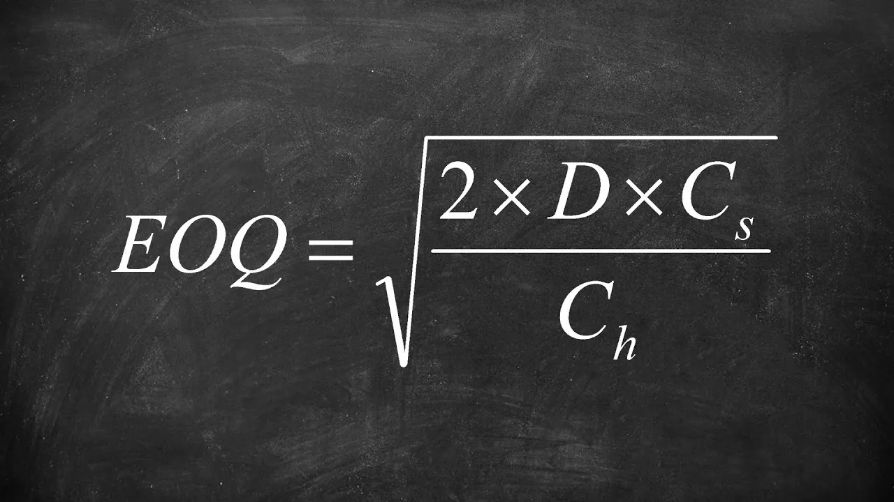 YouTube5:14
Another explanation of Queueing and inventory models.
Queueing and inventory models YouTube8:01
Another explanation of Queueing and inventory models.
Queueing and inventory modelsYouTube7:28Lecture for Queueing and inventory models, compared with the current visual explanation.
Queueing and inventory models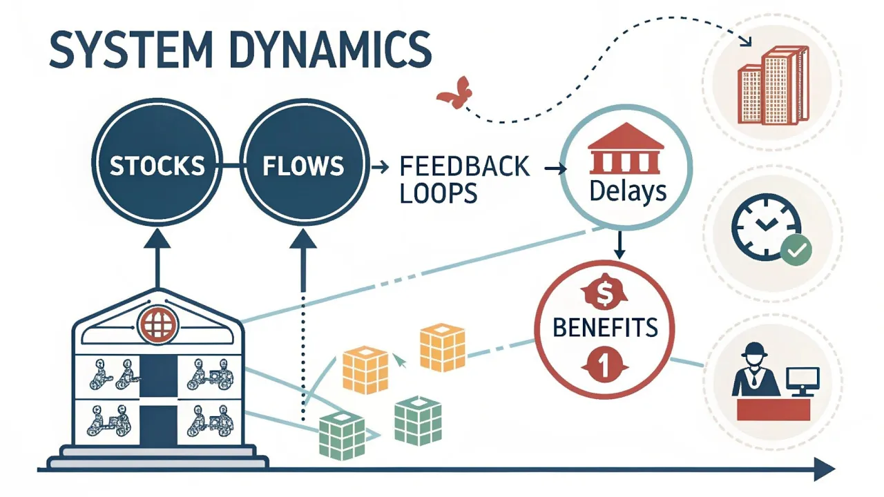 YouTube3:33
Application of Queueing and inventory models, complementing the current explanation.
Queueing and inventory modelsYouTube5:14Lecture for Queueing and inventory models, compared with the current visual explanation.
Queueing and inventory models