Reviewed learning material · Video analysis · EnglishRead the full overview
This 120-second clip introduces a transportation problem with 3 factories and 4 cities, shows the cost/supply/demand table, verifies that total supply equals total demand (125=125), defines the objective as meeting demand while minimizing shipping cost, explains why the Northwest Corner Method starts at the top-left cell, and demonstrates the first allocation of 35 units from Factory 1 to City 1 before ending mid-solution.
This video segment demonstrates the initial steps of solving a balanced transportation problem using the Northwest Corner Method. Starting from the top-left cell, the instructor allocates supplies to meet demands sequentially, updating the remaining supply and demand values and crossing out exhausted rows and columns. The clip covers the complete fulfillment of City 1 and City 2, illustrating the core mechanics of the algorithm.
This 120-second whiteboard segment continues a transportation-problem solution using the Northwest Corner Method. It completes the City 3 column by allocating 20 units from Factory 2 and 10 units from Factory 3, then moves to City 4, skips the exhausted Factory 2 / City 4 cell, and assigns the final 30 units from Factory 3 to City 4. After the allocation table is complete, the narrator explains how to compute total shipping cost by multiplying each allocated quantity by its unit cost and summing the results, writing the expression 35(8)+10(9)+20(12)+20(13)+10(16)+30(5). The clip ends before the final numerical total is evaluated.
This video segment demonstrates the final step of solving a transportation problem using the Northwest Corner Method. It shows a completed allocation table and calculates the total transportation cost by multiplying the allocated quantities by their respective unit costs, resulting in a final cost of $1,180.
Use the learning inspector for key ideas and moments, or open the reading tabs for the complete notes.
Generated from the video's visuals and explanation; not verbatim speech.
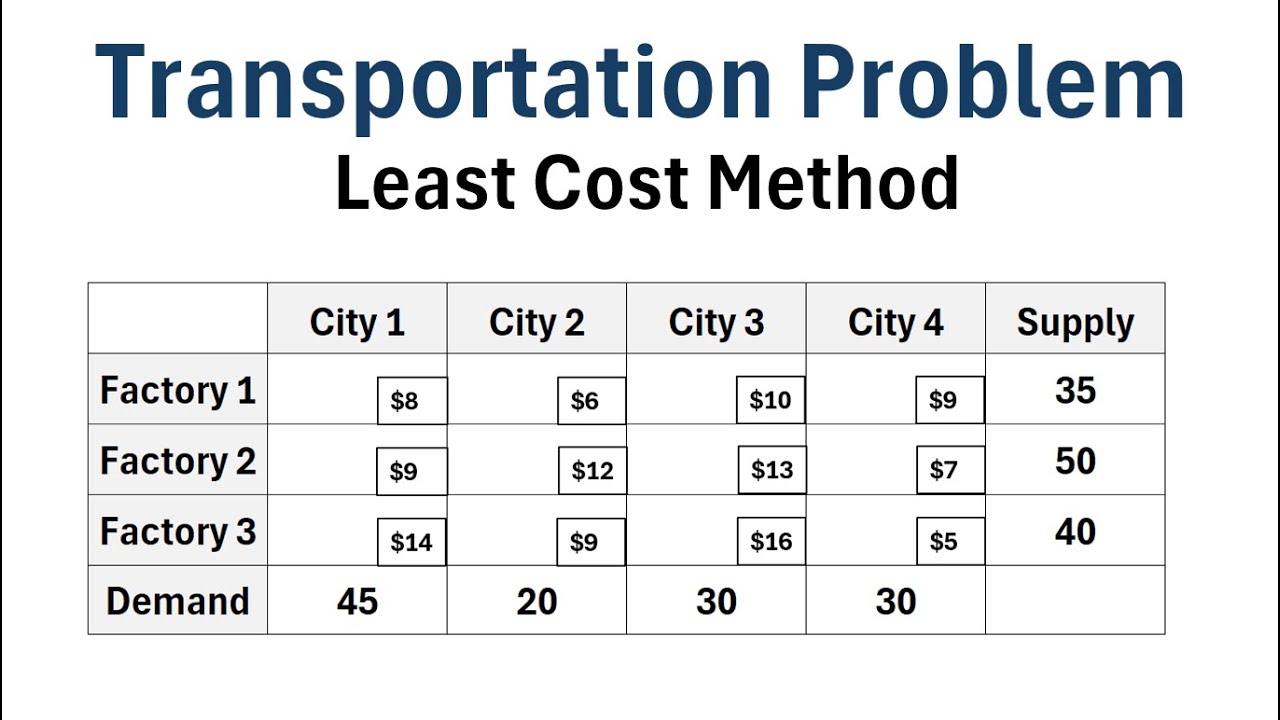
The clip opens by naming the topic: solving a transportation problem with the Northwest Corner Method. On screen, a table lays out 3 factories as rows, 4 cities as columns, unit shipping costs inside, a Supply column on the right, and a Demand row at the bottom.
The presenter reads the marginal totals from the table. Factory supplies are 35, 50, and 40; city demands are 45, 20, 30, and 30. These values define how much each source can send and how much each destination must receive.
Next, the video checks whether the model is balanced. Adding the supply column gives 35+50+40=125, and adding the demand row gives 45+20+30+30=125. Because the two totals match, the speaker identifies this as a balanced transportation problem.
The objective is then stated in words: satisfy every city's demand while minimizing total shipping cost. The interior dollar amounts are interpreted as per-unit costs for shipping from a particular factory to a particular city.
To explain the method name, the presenter draws a compass and points to the northwest direction. This visual analogy translates directly to the table geometry: northwest means the upper-left corner, so the algorithm begins in the top-left cell.
The first worked step applies that rule to the example. The top-left cell is the Factory 1 to City 1 route, whose printed unit cost is $8. City 1 needs 45 units, but Factory 1 only has 35 available, so the clip assigns all 35 units from Factory 1 to City 1 and writes 35 into that cell.
The segment ends while the speaker is still explaining the consequence of using up Factory 1's supply, before showing the updated remaining demand or the next move in the Northwest Corner Method.
The video presents a transportation problem tableau with three factories and four cities. The goal is to find an initial feasible shipping plan using the Northwest Corner Method. We begin at the top-left cell, representing shipments from Factory 1 to City 1.
Factory 1 has a supply of 35 units, while City 1 requires 45 units. Following the method, we allocate the maximum possible amount, which is the minimum of supply and demand: min(35,45)=35. We record 35 in the cell and cross out Factory 1's supply, as it is now exhausted.
City 1's demand is reduced by the allocated amount: 45−35=10. Since there is still unmet demand, we move down to the next available cell in the same column, which corresponds to Factory 2 supplying City 1.
Factory 2 has an initial supply of 50 units. We allocate the remaining demand of 10 units from Factory 2 to City 1. We write 10 in the cell and update Factory 2's remaining supply to 50−10=40. City 1's demand is now fully satisfied.
Because City 1's demand is met, we cross out the remaining empty cell in its column (Factory 3 to City 1). Similarly, because Factory 1's supply was exhausted earlier, we cross out all remaining cells in its row (Factory 1 to Cities 2, 3, and 4).
With the first column and row resolved, we move to the next available cell in the tableau, which is Factory 2 supplying City 2. City 2 has a total demand of 20 units.
Factory 2 currently has 40 units of supply remaining. We allocate the full demand of 20 units from Factory 2 to City 2. We record 20 in the cell and reduce Factory 2's supply to 40−20=20.
City 2's demand is now completely met. We cross out the remaining cell in City 2's column (Factory 3 to City 2). The clip ends here, with Factory 2 having 20 units left to distribute to Cities 3 and 4.
The segment opens with the transportation tableau already partly filled. The narrator states that the current column is finished and the method advances to the next column, City 3, selecting the first available cell there.
The City 3 demand is read directly from the table as 30. Because Factory 2 still has 20 units of supply remaining, the Northwest Corner rule allocates the smaller of remaining supply and remaining demand to the active cell, giving x23=20.
That allocation exhausts Factory 2, so its remaining supply is crossed out. At the same time, City 3's demand is reduced from 30 to 10, showing that the column is not yet complete.
Since demand remains in the same column but the current row is exhausted, the procedure moves downward to the next available row, Factory 3. This is the visual cue that distinguishes row exhaustion from column completion.
Factory 3 begins with 40 units of supply. To satisfy the remaining City 3 demand of 10, the method allocates x33=10, which reduces Factory 3's supply to 30 and completes City 3 demand entirely.
With City 3 finished, the algorithm shifts right to the next column, City 4. The first cell in that column is Factory 2 / City 4, but that cell is not usable because Factory 2 supply was already exhausted earlier.
The narrator therefore crosses out Factory 2 / City 4 and proceeds to the last active cell, Factory 3 / City 4. City 4 demand is 30, and Factory 3 also has exactly 30 units left, so the final allocation is x34=30.
At this point the allocation table is complete. The occupied cells are 35 from Factory 1 to City 1, 10 from Factory 2 to City 1, 20 from Factory 2 to City 2, 20 from Factory 2 to City 3, 10 from Factory 3 to City 3, and 30 from Factory 3 to City 4.
The lesson then turns from feasibility to objective evaluation. The narrator explains that total shipping cost is computed by taking each allocated quantity, multiplying it by the unit shipping cost in the same cell, and adding all such products.
Applying that rule to the displayed solution produces the written expression TOTAL COST = 35(8)+10(9)+20(12)+20(13)+10(16)+30(5). Each term corresponds to one occupied cell in the final Northwest Corner allocation.
The clip ends as the narrator begins to say that entering the expression into a calculator gives the final value, but the numerical total itself is not shown within this segment.
We have successfully applied the Northwest Corner Method to find an initial basic feasible solution for our transportation problem. The table now displays the allocated quantities for each factory-city route, alongside their corresponding unit costs.
To evaluate this solution, we calculate the total transportation cost. This is done by multiplying each allocated quantity by its unit cost and summing these products across all active routes.
Performing the arithmetic: 35 times $8, plus 10 times $9, plus 20 times $12, plus 20 times $13, plus 10 times $16, plus 30 times $5. Adding these values together gives us a total cost of $1,180.
This $1,180 represents the total cost of the current feasible solution obtained through the Northwest Corner Method.
Knowledge cards
01
Transportation problem table
The video represents a transportation problem as a matrix-like table. Rows are factories (sources), columns are cities (destinations), the rightmost column lists each factory's supply, the bottom row lists each city's demand, and the interior cells list unit shipping costs for each factory-city pair.
02
Balanced transportation problem
A transportation problem is balanced when total supply equals total demand. In the example, total supply is 35+50+40=125 and total demand is 45+20+30+30=125, so the problem is balanced.
i∑Supplyi=j∑Demandj
03
Objective of the example
The goal is to meet every city's demand while minimizing total shipping cost. The numbers inside the table are interpreted as dollars per unit shipped along each route.
04
Why it is called the Northwest Corner Method
The speaker uses a compass analogy: northwest corresponds to the upper-left direction. Therefore, the method starts in the top-left cell of the transportation table.
05
First allocation step
Starting at the top-left cell (Factory 1, City 1), the method assigns as much as possible from the current factory to the current city. Since Factory 1 has supply 35 and City 1 has demand 45, the first allocation is 35 units.
x11=min(35,45)=35
06
Northwest Corner Method Overview
A heuristic for finding an initial basic feasible solution in transportation problems. It starts at the top-left (northwest) cell, allocates min(supply,demand), and moves right if supply is exhausted or down if demand is exhausted.
xij=min(Si,Dj)
07
Step 1: Initial Allocation
At cell (Factory 1, City 1), supply is 35 and demand is 45. Allocate min(35,45)=35. Factory 1's supply becomes 0 (crossed out). City 1's remaining demand becomes 45−35=10.
x11=35,S1=0,D1=10
08
Step 2: Moving Down for Unmet Demand
Since City 1 still needs 10 units, move down to cell (Factory 2, City 1). Factory 2 has 50 units. Allocate 10. Factory 2's remaining supply becomes 50−10=40. City 1's demand is now 0.
x21=10,S2=40,D1=0
09
Step 3: Crossing Out Exhausted Rows/Columns
When a row's supply or column's demand reaches zero, all remaining cells in that row/column are crossed out. Here, Factory 1's row and City 1's column are fully crossed out after their respective resources are depleted.
10
Step 4: Proceeding to Next Column
Move to the next available cell, (Factory 2, City 2). City 2 demands 20 units. Factory 2 has 40 units left. Allocate 20. Factory 2's remaining supply drops to 20. City 2's demand is met, so its column is crossed out.
x22=20,S2=20,D2=0
11
Northwest Corner transition into City 3
After finishing the previous column, the method moves to the next column and chooses the first available cell. In this clip, that means entering the City 3 column and preparing to satisfy its demand of 30 units.
12
Allocate 20 from Factory 2 to City 3
Factory 2 has 20 units of remaining supply, while City 3 needs 30. The Northwest Corner rule assigns the smaller amount, so 20 units are placed in the Factory 2 / City 3 cell. This exhausts Factory 2 and leaves 10 units of City 3 demand unmet.
x23=min(20,30)=20
13
Move down when a row is exhausted
Because Factory 2 supply becomes zero but City 3 still needs 10 units, the algorithm does not stop or move right. Instead, it moves downward within the same column to the next available row, Factory 3.
14
Allocate 10 from Factory 3 to City 3
Factory 3 has 40 units available and City 3 still needs 10. The method assigns 10 units to the Factory 3 / City 3 cell, which completes City 3 demand and reduces Factory 3 supply to 30.
x33=min(40,10)=10
15
Move right when a column is satisfied
Once City 3 demand reaches zero, the column is eliminated and the procedure advances to the next column, City 4, even though Factory 3 still has supply remaining.
16
Skip cells in exhausted rows
When entering City 4, the Factory 2 / City 4 cell is crossed out because Factory 2 supply was already used up. Only cells with both remaining row supply and remaining column demand can receive allocations.
17
Final allocation from Factory 3 to City 4
City 4 requires 30 units and Factory 3 has exactly 30 units left. The last active cell therefore receives 30 units, completing the feasible Northwest Corner solution.
x34=min(30,30)=30
18
Completed allocation pattern
The full allocation shown by the end of the procedure is 35 from Factory 1 to City 1, 10 from Factory 2 to City 1, 20 from Factory 2 to City 2, 20 from Factory 2 to City 3, 10 from Factory 3 to City 3, and 30 from Factory 3 to City 4.
19
Total shipping cost rule
To evaluate the transportation solution, multiply each allocated quantity by the unit shipping cost in the same cell and sum all products over the occupied cells.
TOTAL COST=(i,j)∈A∑xijcij
20
Cost expression for this example
Using the allocated cells and their unit costs, the written objective expression is 35 times 8 plus 10 times 9 plus 20 times 12 plus 20 times 13 plus 10 times 16 plus 30 times 5. The clip ends before the final numeric total is computed.
TOTAL COST=35(8)+10(9)+20(12)+20(13)+10(16)+30(5)
21
Total Cost Calculation in Transportation Problems
After finding an initial feasible solution (such as with the Northwest Corner Method), the total cost is evaluated by summing the product of the allocated quantity and the unit cost for every occupied cell in the transportation tableau. Formula: Total Cost = ∑ (Allocation × Unit Cost).
i,j∑xijcij
22
Northwest Corner Method Overview
The Northwest Corner Method is a heuristic used to generate an initial basic feasible solution for a transportation problem. It starts allocating from the top-left (northwest) cell of the cost matrix, satisfying supply and demand constraints sequentially without considering the unit costs during the allocation phase.
Detailed learning notes
Explore conditions, steps and evidence. Supplementary explanations are labeled separately from content shown in the video.
Symbols · 37
Factory i
Clear evidence
Shown in the video
Evidence
Diagram
Observation
Rows are labeled Factory 1, Factory 2, Factory 3.
Audio
Observation
The speaker says there are three factories that produce some good.
Symbol
Factory i
Meaning
Production source or origin in the transportation table.
Domain
i∈ \{1,2,3\}
City j
Clear evidence
Shown in the video
Evidence
Diagram
Observation
Columns are labeled City 1, City 2, City 3, City 4.
Audio
Observation
The speaker says there are four cities that have a demand for that good.
Symbol
City j
Meaning
Destination or demand point in the transportation table.
Domain
j∈ \{1,2,3,4\}
Supply_i
Clear evidence
Shown in the video
Evidence
Diagram
Observation
Rightmost column header is Supply with values 35, 50, 40.
Audio
Observation
Factory 1 has a total supply of 35; Factory 2 makes 50 units; Factory 3 makes 40 units.
Symbol
Supply_i
Meaning
Total units available from factory i.
Domain
Units of goods
Demand_j
Clear evidence
Shown in the video
Evidence
Diagram
Observation
Bottom row header is Demand with values 45, 20, 30, 30.
Audio
Observation
City 1 has a total demand of 45 units; City 2 has 20; City 3 has 30; City 4 has 30.
Symbol
Demand_j
Meaning
Total units required by city j.
Domain
Units of goods
Cost_{ij}
Clear evidence
Shown in the video
Evidence
Diagram
Observation
Interior cells contain dollar amounts such as $8, $6, $10, $9, $12, $13, $7, $14, $16, $5.
Audio
Observation
Within each of these cells in the table, I've shown the shipping costs per unit.
Symbol
Cost_{ij}
Meaning
Shipping cost per unit from factory i to city j.
Domain
Dollars per unit
∑i Supply_i
Clear evidence
Shown in the video
Evidence
Diagram
Observation
The speaker writes 125 beside the Supply column after circling 35, 50, 40.
Audio
Observation
If you add up these values, that turns out to be 125.
Symbol
∑i Supply_i
Meaning
Total supply across all factories.
Domain
Units of goods
∑j Demand_j
Clear evidence
Shown in the video
Evidence
Diagram
Observation
The speaker writes 125 below the Demand row after circling 45, 20, 30, 30.
Audio
Observation
The total demand among all four cities is also 125.
Symbol
∑j Demand_j
Meaning
Total demand across all cities.
Domain
Units of goods
x11
Clear evidence
Shown in the video
Evidence
Diagram
Observation
The top-left cell (Factory 1, City 1) is circled and then 35 is written inside it.
Audio
Observation
This factory has a supply of 35, so we can use up all 35 of those units.
Uncertainties
The clip ends before the method states the full allocation rule or updates remaining demand.
Symbol
x11
Meaning
Quantity shipped from Factory 1 to City 1 under the Northwest Corner Method.
Domain
Units of goods
Factory 1
Clear evidence
Shown in the video
Evidence
Diagram
Observation
Row label 'Factory 1' in the transportation table.
Symbol
Factory 1
Meaning
First supply source with an initial capacity of 35 units.
Domain
Supply source
Factory 2
Clear evidence
Shown in the video
Evidence
Diagram
Observation
Row label 'Factory 2' in the transportation table.
Symbol
Factory 2
Meaning
Second supply source with an initial capacity of 50 units.
Domain
Supply source
Factory 3
Clear evidence
Shown in the video
Evidence
Diagram
Observation
Row label 'Factory 3' in the transportation table.
Symbol
Factory 3
Meaning
Third supply source with an initial capacity of 40 units.
Domain
Supply source
City 1
Clear evidence
Shown in the video
Evidence
Diagram
Observation
Column label 'City 1' in the transportation table.
Symbol
City 1
Meaning
First demand destination requiring 45 units.
Domain
Demand destination
Knowledge points · 15
Transportation problem setup
Clear evidence
Shown in the video
Evidence
Audio
Observation
In this video, I will explain how to solve the transportation problem using the Northwest Corner Method.
Diagram
Observation
A table shows factories as rows, cities as columns, interior unit costs, a Supply column, and a Demand row.
Definition
Explanation
The video introduces a transportation problem as a table-based model with multiple production sources and multiple destinations. Rows represent factories, columns represent cities, the rightmost column gives each factory's available supply, the bottom row gives each city's required demand, and the interior cells give unit shipping costs between each factory-city pair.
Formula
Conditions
There are m sources and n destinations.
Each source has a supply amount.
Each destination has a demand amount.
Each source-destination pair has a unit shipping cost.
Balanced transportation problem
Clear evidence
Shown in the video
Evidence
Audio
Observation
So this is known as a balanced transportation problem.
Diagram
Observation
The speaker sums the Supply column to 125 and the Demand row to 125.
Definition
Explanation
A transportation problem is called balanced when total supply equals total demand. In the example, total supply is 35+50+40=125 and total demand is 45+20+30+30=125, so the model is balanced.
Formula
i∑Supplyi=j∑Demandj
Conditions
All supplies and demands are nonnegative.
Equality is checked after summing all row supplies and all column demands.
Prerequisites
Transportation problem setup
Objective of the transportation problem
Clear evidence
Shown in the video
Evidence
Audio
Observation
We want to meet the demand of each city, but we want to minimize the shipping costs.
Diagram
Observation
Interior cells contain per-unit costs such as $8 from Factory 1 to City 1 and $6 from Factory 1 to City 2.
Definition
Explanation
The goal stated in the clip is to satisfy every city's demand while minimizing total shipping cost. The table entries are interpreted as costs per unit shipped from a given factory to a given city.
Formula
Conditions
Demand must be met at each destination.
Costs are linear per unit in the displayed setup.
Prerequisites
Transportation problem setup
Meaning of "Northwest" in the method name
Clear evidence
Shown in the video
Evidence
Audio
Observation
If you imagine that we draw a compass ... northwest would be in this direction ... pointing to the top left.
Diagram
Observation
A compass with N, S, E, W is drawn, and an arrow indicates the northwest direction.
Definition
Explanation
The speaker explains the name by comparing the table to a compass. Northwest corresponds to the upper-left direction, so the method starts at the top-left cell of the transportation table.
Formula
Conditions
The table is oriented with rows increasing downward and columns increasing rightward.
Prerequisites
Transportation problem setup
Starting cell of the Northwest Corner Method
Clear evidence
Shown in the video
Evidence
Audio
Observation
When we use this method, we're always going to start with the cell in the top left corner of the table.
Diagram
Observation
The cell (Factory 1, City 1), containing $8, is circled.
Method
Explanation
The first step of the Northwest Corner Method is to begin in the top-left cell of the transportation table. In this example, that is the Factory 1 to City 1 cell with unit cost $8.
Formula
Conditions
Use the current active subtable's top-left cell.
The method proceeds cell by cell from that starting position.
Prerequisites
Meaning of "Northwest" in the method name
Transportation problem setup
First allocation step in the example
Approximate timing
Shown in the video
Evidence
Audio
Observation
City 1 has a total demand of 45 units. So we're going to fulfill as much of that demand as possible in this cell right here based on whatever the supply is for this factory.
Diagram
Observation
The speaker circles City 1 demand 45, Factory 1 supply 35, and writes 35 into the (Factory 1, City 1) cell.
Uncertainties
The clip ends before the general min(supply, demand) rule is fully stated or the remaining demand update is shown.
Method
Explanation
At the starting cell, the video allocates as much as possible from the chosen factory to the chosen city, limited by that factory's available supply. Here Factory 1 has supply 35 and City 1 needs 45, so all 35 units from Factory 1 are assigned to City 1.
Formula
x11=min(35,45)=35
Conditions
Compare the current row supply and current column demand.
Assign the smaller available amount to the current cell.
This clip only demonstrates the case where supply is smaller than demand.
Prerequisites
Starting cell of the Northwest Corner Method
Transportation problem setup
Northwest Corner Method for Transportation Problems
Clear evidence
Shown in the video
Evidence
Audio
Observation
The speaker explains the process of fulfilling demand by moving down or right based on remaining supply and demand, which is characteristic of the Northwest Corner Method.
Method
Explanation
A heuristic algorithm used to find an initial basic feasible solution for a transportation problem. It starts at the top-left (northwest) cell of the transportation tableau and allocates as much as possible to that cell, then moves either down or right depending on whether supply or demand is exhausted, repeating until all supplies and demands are met.
Formula
Conditions
Total supply must equal total demand (balanced problem).
Start allocation at the top-left cell.
Allocate min(remaining supply, remaining demand) to the current cell.
Move right if supply is exhausted; move down if demand is exhausted.
If both are exhausted simultaneously, move right (or down) and allocate 0 to the next cell to maintain degeneracy rules.
Northwest Corner transition to the next column
Clear evidence
Shown in the video
Evidence
Audio
Observation
The narrator says, "So now we're done with this column, we'll move on to the next column, so city three."
Diagram
Observation
The active focus shifts from the completed City 2 column to the first available cell in the City 3 column.
Method
Explanation
When a column's demand has been fully satisfied, the method advances to the next column and selects the next available cell in that column. In this clip, after finishing City 2, the process moves to City 3 and identifies the first usable cell there.
Formula
Conditions
The current column's demand is already met.
The next column still has unmet demand.
The chosen cell must not already be eliminated by exhausted supply or demand.
Exhausting a row forces movement downward
Clear evidence
Shown in the video
Evidence
Audio
Observation
The narrator says Factory 2 has 20 supply left, uses all of it, then notes there is still 10 demand left and they need to move down to the next cell.
Formula
Observation
The Factory 2 / City 3 cell receives 20, the Factory 2 supply is exhausted, and the City 3 demand is reduced from 30 to 10.
Method
Explanation
If the selected cell consumes all remaining supply in the current row but the column demand is not yet met, the algorithm eliminates that row and moves down to the next available row in the same column. Here, allocating 20 from Factory 2 to City 3 exhausts Factory 2, leaving 10 units of City 3 demand to be satisfied from Factory 3.
Formula
Conditions
The current row's remaining supply is less than the current column's remaining demand.
After allocation, the row supply becomes zero.
The column demand remains positive.
Prerequisites
Northwest Corner transition to the next column
Satisfying a column forces movement to the next column
Clear evidence
Shown in the video
Evidence
Audio
Observation
The narrator says Factory 3 has supply 40, takes 10 from there, reduces supply to 30, puts 10 in the cell, and then states that City 3 is now done so they move to the next column, City 4.
Formula
Observation
The Factory 3 / City 3 cell receives 10, the City 3 demand becomes fully satisfied, and the focus shifts to City 4.
Method
Explanation
If the selected cell consumes exactly the remaining demand in the current column while supply remains in the row, the algorithm eliminates that column and moves right to the next column. In this clip, allocating 10 from Factory 3 to City 3 completes City 3 demand, so the process advances to City 4 while Factory 3 still has 30 units left.
Formula
Conditions
The current column's remaining demand is less than or equal to the current row's remaining supply.
After allocation, the column demand becomes zero.
The row supply may remain positive.
Prerequisites
Exhausting a row forces movement downward
Skipping cells whose row supply is already exhausted
Clear evidence
Shown in the video
Evidence
Audio
Observation
The narrator says, "We can see that we've already exhausted the supply of factory two, so we actually just need to cross this cell out, and then we'll move to this very last cell."
Diagram
Observation
The Factory 2 / City 4 cell is crossed out before attention moves to Factory 3 / City 4.
Method
Explanation
When moving into a new column, any cell in a row whose supply has already been used up is not eligible for allocation. The method crosses out that cell and proceeds to the next available cell in the column. Here, Factory 2 / City 4 is skipped because Factory 2 supply was exhausted earlier.
Formula
Conditions
The row supply is already zero.
The cell lies in the currently active column.
Another row in the same column still has available supply.
Prerequisites
Exhausting a row forces movement downward
Final allocation satisfies the last column
Clear evidence
Shown in the video
Evidence
Audio
Observation
The narrator says the total demand for City 4 is 30 and that they can meet it using the remaining supply, putting 30 units in the last cell.
Formula
Observation
The Factory 3 / City 4 cell receives 30, and the remaining Factory 3 supply becomes 0.
Method
Explanation
At the last active cell, the remaining supply is assigned to the remaining demand. In this example, Factory 3 still has 30 units and City 4 needs 30 units, so the final allocation is 30 from Factory 3 to City 4, completing the feasible Northwest Corner solution.
Formula
Conditions
Only one active cell remains.
The remaining row supply equals the remaining column demand in this example.
All previous rows and columns have been eliminated or satisfied.
Prerequisites
Skipping cells whose row supply is already exhausted
Claims and conditions · 9
The example is a balanced transportation problem
Clear evidence
Shown in the video
Evidence
Audio
Observation
The total supply ... turns out to be 125 ... the total demand ... is also 125. So this is known as a balanced transportation problem.
Diagram
Observation
125 is written next to the Supply column and again below the Demand row.
Proposition
Statement
For the displayed 3-by-4 example, total supply equals total demand, both being 125, so the transportation problem is balanced.
Hypotheses
Supply values are 35, 50, 40.
Demand values are 45, 20, 30, 30.
Quantifiers
For this specific example table.
Northwest Corner Method starts at the top-left cell
Clear evidence
Shown in the video
Evidence
Audio
Observation
When we use this method, we're always going to start with the cell in the top left corner of the table.
Diagram
Observation
The top-left interior cell is circled.
Proposition
Statement
Using the Northwest Corner Method, the initial allocation is made in the top-left cell of the transportation table.
Hypotheses
The transportation table is arranged with sources as rows and destinations as columns.
Quantifiers
For the method as introduced in this clip.
City 3 demand equals 30
Clear evidence
Shown in the video
Evidence
Audio
Observation
The narrator states that City 3 has a total demand of 30.
Formula
Observation
The Demand row under City 3 shows 30.
Proposition
Statement
The destination City 3 requires 30 units in this transportation table.
Hypotheses
The table shown is the active transportation problem instance.
The bottom row labeled Demand lists destination requirements.
Quantifiers
For the specific City 3 column in the displayed table.
Factory 2 has 20 units of supply remaining before serving City 3
Clear evidence
Shown in the video
Evidence
Audio
Observation
The narrator says Factory 2 has 20 supply left.
Formula
Observation
The Factory 2 Supply entry shows 50 crossed out, 40 crossed out, and 20 written as the remaining amount.
Proposition
Statement
At the moment the algorithm enters the City 3 column, Factory 2 still has 20 units available.
Hypotheses
Earlier allocations from Factory 2 to City 1 and City 2 have already been made.
The Supply column tracks remaining capacity after each allocation.
Quantifiers
For Factory 2 at the start of the City 3 allocation step.
After allocating 20 from Factory 2, City 3 still needs 10 units
Clear evidence
Shown in the video
Evidence
Audio
Observation
The narrator says a total of 20 of the 30 demand has been met, so the demand is reduced by 20 and becomes 10.
Formula
Observation
The City 3 demand entry changes from 30 to 10 after writing 20 in the Factory 2 / City 3 cell.
Proposition
Statement
The residual demand at City 3 after the Factory 2 allocation is 10 units.
Hypotheses
City 3 initial demand is 30.
The allocation x23=20 is made from Factory 2 to City 3.
Quantifiers
For City 3 immediately after the Factory 2 / City 3 allocation.
Using 10 units from Factory 3 leaves 30 units remaining
Clear evidence
Shown in the video
Evidence
Audio
Observation
The narrator says Factory 3 has a supply of 40, they take 10 from there, and reduce the supply to 30.
Formula
Observation
The Factory 3 Supply entry changes from 40 to 30 when 10 is placed in the Factory 3 / City 3 cell.
Proposition
Statement
After allocating 10 units from Factory 3 to City 3, Factory 3's remaining supply is 30 units.
Hypotheses
Factory 3 initial supply is 40.
The allocation x33=10 is made.
Quantifiers
For Factory 3 immediately after the Factory 3 / City 3 allocation.
City 4 demand equals 30
Clear evidence
Shown in the video
Evidence
Audio
Observation
The narrator says the total demand for City 4 is 30.
Formula
Observation
The Demand row under City 4 shows 30.
Proposition
Statement
The destination City 4 requires 30 units in this transportation table.
Hypotheses
The table shown is the active transportation problem instance.
The bottom row labeled Demand lists destination requirements.
Quantifiers
For the specific City 4 column in the displayed table.
The final allocation is 30 units from Factory 3 to City 4
Clear evidence
Shown in the video
Evidence
Audio
Observation
The narrator says they will use the remaining supply and put 30 units in this cell to meet City 4 demand.
Formula
Observation
The Factory 3 / City 4 cell receives 30, and the remaining Factory 3 supply becomes 0.
Proposition
Statement
In the completed Northwest Corner solution, x34=30.
Hypotheses
Factory 3 has 30 units remaining after serving City 3.
City 4 still needs 30 units.
Factory 2 supply is exhausted, so Factory 2 / City 4 is skipped.
Quantifiers
For the last active cell in the displayed solution.
Total cost expression for the displayed allocation
Clear evidence
Shown in the video
Evidence
Formula
Observation
The board writes TOTAL COST: 35($8)+10($9)+20($12)+20($13)+10($16)+30($5).
Audio
Observation
The narrator reads each allocated cell and multiplies its quantity by the unit shipping price.
Uncertainties
The final numeric total is not shown within this clip.
Proposition
Statement
The total shipping cost for the allocation shown is expressed as 35 times 8 plus 10 times 9 plus 20 times 12 plus 20 times 13 plus 10 times 16 plus 30 times 5.
Hypotheses
The allocated cells are (1,1), (2,1), (2,2), (2,3), (3,3), and (3,4).
The corresponding unit costs are 8, 9, 12, 13, 16, and 5.
Quantifiers
For the specific completed allocation table shown in the clip.
Derivations and proofs · 9
Verification that the example is balanced
Clear evidence
Shown in the video
Evidence
Audio
Observation
If you add up these values, that turns out to be 125 ... the total demand ... is also 125.
Diagram
Observation
The Supply entries 35, 50, 40 are circled and 125 is written; the Demand entries 45, 20, 30, 30 are circled and 125 is written.
Numerical verification
Steps
Expression
35+50+40=125
Explanation
Add the three factory supplies shown in the Supply column.
Justification
Direct summation of the displayed supply values.
Shown in the video
Expression
45+20+30+30=125
Explanation
Add the four city demands shown in the Demand row.
Justification
Direct summation of the displayed demand values.
Shown in the video
Expression
125=125
Explanation
Compare total supply with total demand.
Justification
Equality of the two totals identifies the model as balanced.
Shown in the video
Conclusion
Total supply equals total demand, so the example is a balanced transportation problem.
First allocation under the Northwest Corner Method
Approximate timing
Shown in the video
Evidence
Audio
Observation
City 1 has a total demand of 45 units ... this factory has a supply of 35, so we can use up all 35 of those units.
Diagram
Observation
The (Factory 1, City 1) cell is selected and 35 is written into it.
Uncertainties
The clip stops before the remaining demand for City 1 is updated or the next move is explained.
Intuitive argument
Steps
Expression
Start at (Factory1,City1)
Explanation
Begin in the top-left cell of the transportation table.
Justification
Stated rule of the Northwest Corner Method in the clip.
Shown in the video
Expression
Supply1=35,Demand1=45
Explanation
Read the row supply and column demand relevant to the starting cell.
Justification
Values are explicitly shown in the table and spoken aloud.
Shown in the video
Expression
x11=35
Explanation
Allocate all available supply from Factory 1 to City 1 because the supply is smaller than the demand.
Justification
The speaker says to fulfill as much demand as possible based on the factory's supply.
Shown in the video
Conclusion
The first Northwest Corner allocation in this example is 35 units from Factory 1 to City 1.
Allocation Process for City 1 and Factory 1
Clear evidence
Shown in the video
Evidence
Audio
Observation
Speaker narrates crossing out 35, updating demand to 10, moving down to Factory 2, allocating 10, updating supply to 40, and crossing out remaining cells in City 1 and Factory 1.
Animation
Observation
Visual updates of numbers and crossing out of cells in the first column and first row.
Visual argument
Steps
Expression
x11=min(35,45)=35
Explanation
Allocate the maximum possible amount from Factory 1 to City 1.
Subtract allocated amount from Factory 2's current supply.
Shown in the video
Expression
D2=20−20=0
Explanation
City 2's demand is fully satisfied.
Justification
Remaining demand becomes zero.
Shown in the video
Expression
x32=0
Explanation
Cross out the remaining cell in City 2's column.
Justification
Demand for City 2 is met, so no further allocations can be made to this column.
Shown in the video
Conclusion
The second column (City 2) is resolved, leaving Factory 2 with 20 units of supply and Cities 3 and 4 with unmet demands.
First allocation in the City 3 column
Clear evidence
Shown in the video
Evidence
Audio
Observation
The narrator explains that City 3 demand is 30, Factory 2 has 20 supply left, they use all of it, write 20 in the cell, and reduce City 3 demand to 10.
Formula
Observation
The Factory 2 / City 3 cell is filled with 20; Factory 2 supply goes from 20 to 0; City 3 demand goes from 30 to 10.
Visual argument
Steps
Expression
d3=30
Explanation
Read the remaining demand for City 3 from the Demand row.
Justification
The table explicitly shows 30 under City 3, and the narrator states this value.
Shown in the video
Expression
s2left=20
Explanation
Read the remaining supply for Factory 2 before entering the City 3 column.
Justification
The Supply column for Factory 2 shows 20 after earlier allocations, and the narrator says Factory 2 has 20 supply left.
Shown in the video
Expression
x23=min(s2left,d3)=min(20,30)=20
Explanation
Allocate the smaller of remaining supply and remaining demand to the current Northwest Corner cell.
Justification
This is the Northwest Corner rule demonstrated by the narrator when they say to use up all remaining supply from Factory 2.
Derived from the video
Expression
s2new=20−20=0
Explanation
Subtract the allocated amount from Factory 2's remaining supply.
Justification
The board crosses out the Factory 2 supply value after placing 20 in the cell.
Shown in the video
Expression
d3new=30−20=10
Explanation
Subtract the allocated amount from City 3's remaining demand.
Justification
The narrator explicitly says the demand is reduced by 20 and becomes 10, and the table updates accordingly.
Shown in the video
Conclusion
After the first City 3 step, 20 units are shipped from Factory 2 to City 3, Factory 2 is exhausted, and City 3 still needs 10 units.
Second allocation in the City 3 column
Clear evidence
Shown in the video
Evidence
Audio
Observation
The narrator says there is still 10 demand left, so they move down to the next cell and use Factory 3, taking 10 from its supply of 40 and reducing supply to 30.
Formula
Observation
The Factory 3 / City 3 cell is filled with 10; Factory 3 supply goes from 40 to 30; City 3 demand is completed.
Visual argument
Steps
Expression
d3left=10
Explanation
Carry forward the unmet demand at City 3 from the previous step.
Justification
The previous derivation ended with City 3 demand reduced to 10, and the narrator repeats that 10 demand remains.
Shown in the video
Expression
s3=40
Explanation
Read Factory 3's available supply before this allocation.
Justification
The Supply column for Factory 3 shows 40, and the narrator states this value.
Shown in the video
Expression
x33=min(s3,d3left)=min(40,10)=10
Explanation
Allocate the smaller of remaining supply and remaining demand to the new active cell.
Justification
This follows the same Northwest Corner rule used by the narrator when they say to take 10 from Factory 3.
Derived from the video
Expression
s3new=40−10=30
Explanation
Subtract the allocated amount from Factory 3's supply.
Justification
The board updates Factory 3's remaining supply to 30, and the narrator says they reduce the supply to 30.
Shown in the video
Expression
d3new=10−10=0
Explanation
Subtract the allocated amount from City 3's remaining demand.
Justification
The narrator states that the total demand has now been met, so City 3 is done.
Shown in the video
Conclusion
After the second City 3 step, 10 units are shipped from Factory 3 to City 3, City 3 demand is fully satisfied, and Factory 3 retains 30 units of supply.
Allocation in the City 4 column
Clear evidence
Shown in the video
Evidence
Audio
Observation
The narrator says City 3 is done, so they move to City 4; Factory 2 supply is exhausted so that cell is crossed out; City 4 demand is 30 and is met using the remaining supply in the last cell.
Formula
Observation
The Factory 2 / City 4 cell is crossed out, then the Factory 3 / City 4 cell receives 30 and Factory 3 supply becomes 0.
Visual argument
Steps
Expression
move to City 4
Explanation
Advance to the next column once City 3 demand is fully satisfied.
Justification
The narrator explicitly says that since City 3 is done, they move to the next column, City 4.
Shown in the video
Expression
x24is not allowed
Explanation
Skip the Factory 2 / City 4 cell because Factory 2 supply is already exhausted.
Justification
The narrator says they have already exhausted the supply of Factory 2 and crosses out that cell.
Shown in the video
Expression
d4=30
Explanation
Read the remaining demand for City 4 from the Demand row.
Justification
The table shows 30 under City 4, and the narrator states the total demand for City 4 is 30.
Shown in the video
Expression
s3left=30
Explanation
Use the remaining supply at Factory 3 after the City 3 allocation.
Justification
The previous derivation ended with Factory 3 having 30 units left, and the narrator refers to the remaining supply.
Shown in the video
Expression
x34=min(s3left,d4)=min(30,30)=30
Explanation
Allocate the smaller of remaining supply and remaining demand to the final active cell.
Justification
This matches the narrator's instruction to put 30 units in the last cell to meet City 4 demand.
Derived from the video
Expression
s3new=30−30=0
Explanation
Subtract the allocated amount from Factory 3's remaining supply.
Justification
The board updates Factory 3's supply to 0 after placing 30 in the Factory 3 / City 4 cell.
Shown in the video
Expression
d4new=30−30=0
Explanation
Subtract the allocated amount from City 4's demand.
Justification
The narrator says this meets the demand for City 4, and the table marks the column complete.
Shown in the video
Conclusion
The final active allocation is 30 units from Factory 3 to City 4, which exhausts both Factory 3 supply and City 4 demand and completes the Northwest Corner solution.
Constructing the total shipping cost expression
Clear evidence
Shown in the video
Evidence
Audio
Observation
The narrator explains that total shipping cost is found by multiplying the units in each allocated cell by the unit shipping price and adding the results.
Formula
Observation
The board writes TOTAL COST: 35($8)+10($9)+20($12)+20($13)+10($16)+30($5).
Uncertainties
The clip ends before the final arithmetic total is written or spoken.
Identify every cell that received a nonzero allocation in the completed table.
Justification
These are exactly the cells visibly filled in the final allocation grid.
Shown in the video
Expression
35×8
Explanation
Multiply the allocation in Factory 1 / City 1 by its unit cost.
Justification
The narrator reads this first allocated cell and states 35 times 8.
Shown in the video
Expression
10×9
Explanation
Multiply the allocation in Factory 2 / City 1 by its unit cost.
Justification
The narrator identifies the next allocated cell as 10 units with a shipping cost of $9 per unit.
Shown in the video
Expression
20×12
Explanation
Multiply the allocation in Factory 2 / City 2 by its unit cost.
Justification
The narrator reads the next allocated cell as 20 units times $12.
Shown in the video
Expression
20×13
Explanation
Multiply the allocation in Factory 2 / City 3 by its unit cost.
Justification
The narrator reads the next allocated cell as 20 times $13.
Shown in the video
Expression
10×16
Explanation
Multiply the allocation in Factory 3 / City 3 by its unit cost.
Justification
The narrator reads the next allocated cell as 10 times $16.
Shown in the video
Expression
30×5
Explanation
Multiply the allocation in Factory 3 / City 4 by its unit cost.
Justification
The narrator reads the last allocated cell as 30 times $5.
Shown in the video
Expression
TOTAL COST=35(8)+10(9)+20(12)+20(13)+10(16)+30(5)
Explanation
Add all six products to form the objective-value expression.
Justification
This is exactly what the narrator describes and what is written on the board.
Shown in the video
Conclusion
The total shipping cost for the displayed Northwest Corner solution is represented by the sum 35(8)+10(9)+20(12)+20(13)+10(16)+30(5); the final numeric evaluation is not shown in this clip.
Calculation of Total Transportation Cost
Clear evidence
Shown in the video
Evidence
Formula
Observation
The step-by-step arithmetic is shown: 35($8) + 10($9) + 20($12) + 20($13) + 10($16) + 30($5) = $1,180.
Numerical verification
Steps
Expression
35(8)+10(9)+20(12)+20(13)+10(16)+30(5)
Explanation
Multiply each allocated quantity by its corresponding unit cost based on the filled cells in the transportation table.
Justification
Definition of total cost in a transportation problem.
Shown in the video
Expression
280+90+240+260+160+150
Explanation
Compute the individual products for each route.
Justification
Arithmetic multiplication.
Derived from the video
Expression
1180
Explanation
Sum the individual route costs to get the total cost.
Justification
Arithmetic addition.
Shown in the video
Conclusion
The total transportation cost for the given allocation is $1,180.
Worked examples · 4
Worked setup and first step of a transportation problem
Clear evidence
Shown in the video
Evidence
Diagram
Observation
A 3-by-4 transportation table is shown with factories, cities, unit costs, supply, and demand.
Audio
Observation
Let's say we have three factories ... and four cities ... Factory 1 has a total supply of 35 ... City 1 has a total demand of 45 units.
Uncertainties
Only the first allocation step is completed within the clip; the rest of the Northwest Corner solution is not shown.
Problem
Given three factories and four cities with unit shipping costs, supplies, and demands, set up the transportation problem and begin solving it by the Northwest Corner Method.
Interpret the table layout as a transportation matrix.
Justification
Explicitly described by the speaker and visible in the diagram.
Shown in the video
Expression
35+50+40=125
Explanation
Sum the supplies.
Justification
Shown by circling the Supply column and writing 125.
Shown in the video
Expression
45+20+30+30=125
Explanation
Sum the demands.
Justification
Shown by circling the Demand row and writing 125.
Shown in the video
Expression
Balanced because 125=125
Explanation
Conclude the example is balanced.
Justification
Stated directly in the audio.
Shown in the video
Expression
Start at top-left cell (Factory1,City1)
Explanation
Apply the Northwest Corner starting rule.
Justification
Stated directly in the audio and marked visually.
Shown in the video
Expression
x11=35
Explanation
Allocate 35 units from Factory 1 to City 1.
Justification
The speaker says to use up all 35 units of Factory 1's supply toward City 1's demand.
Shown in the video
Answer
The example is a balanced transportation problem, and the first Northwest Corner allocation is 35 units from Factory 1 to City 1.
Verification
Balance is verified by comparing total supply 125 with total demand 125; the first allocation is verified by comparing supply 35 and demand 45 and assigning the smaller amount, 35.
Transportation Problem Example
Clear evidence
Shown in the video
Evidence
Diagram
Observation
A 3x4 transportation table with specific supply and demand values.
Problem
Find an initial basic feasible solution for a transportation problem with 3 factories (supplies: 35, 50, 40) and 4 cities (demands: 45, 20, 30, 30) using the Northwest Corner Method.
Given
Factory 1 supply = 35
Factory 2 supply = 50
Factory 3 supply = 40
City 1 demand = 45
City 2 demand = 20
City 3 demand = 30
City 4 demand = 30
Goal
Determine the allocation amounts for each factory-city pair starting from the northwest corner.
Steps
Expression
x11=35,x21=10
Explanation
Fulfill City 1's demand of 45 using all of Factory 1's supply (35) and 10 units from Factory 2.
Justification
Northwest Corner Method allocation rules.
Shown in the video
Expression
x22=20
Explanation
Fulfill City 2's demand of 20 using the remaining supply of Factory 2.
Justification
Northwest Corner Method allocation rules.
Shown in the video
Answer
Partial allocations found: x11=35, x21=10, x22=20. Factory 2 has 20 units remaining. The process continues for Cities 3 and 4.
Verification
Total allocated so far equals the sum of fulfilled demands (45+20=65). Total supply used equals 35(F1)+30(F2)=65. Balance is maintained.
Completing a Northwest Corner transportation allocation and forming the cost expression
Clear evidence
Shown in the video
Evidence
Audio
Observation
The narrator walks through the remaining steps of a transportation problem using the Northwest Corner Method, then computes the total shipping cost expression.
Formula
Observation
The board shows a 3-by-4 transportation table with factories, cities, supplies, demands, unit costs, allocations, and a TOTAL COST expression.
Uncertainties
The final numerical total cost is not reached within the clip.
Some pre-existing allocations in City 1 and City 2 are only partially explained because they were completed before this segment.
Problem
Continue solving the displayed transportation problem from the City 3 column onward using the Northwest Corner Method, then write the total shipping cost for the resulting allocation.
Given
Factories: Factory 1, Factory 2, Factory 3.
Cities: City 1, City 2, City 3, City 4.
Initial supplies shown in the table: Factory 1=35, Factory 2=50, Factory 3=40.
Initial demands shown in the table: City 1=45, City 2=20, City 3=30, City 4=30.
Unit costs visible in the table include $8, $9, $12, $13, $16, and $5 for the allocated cells used later.
Earlier allocations already present before this clip include 35 from Factory 1 to City 1, 10 from Factory 2 to City 1, and 20 from Factory 2 to City 2.
Goal
Determine the remaining allocations for City 3 and City 4.;State the completed allocation pattern.;Write the total shipping cost expression for the full solution.
Steps
Expression
x23=20
Explanation
Enter the City 3 column, see that City 3 needs 30 units, and allocate all 20 remaining units from Factory 2 to City 3.
Justification
The narrator says Factory 2 has 20 supply left and uses all of it in the next available cell.
Shown in the video
Expression
d3left=10
Explanation
Reduce City 3 demand from 30 to 10 after receiving 20 units.
Justification
The board updates the City 3 demand entry and the narrator explicitly states the reduction.
Shown in the video
Expression
x33=10
Explanation
Move down to Factory 3 in the same column and allocate 10 units from Factory 3 to City 3 to satisfy the remaining demand.
Justification
The narrator says there is still 10 demand left and they meet it using Factory 3.
Shown in the video
Expression
s3left=30
Explanation
Reduce Factory 3 supply from 40 to 30 after sending 10 units to City 3.
Justification
The board updates the Factory 3 supply entry and the narrator states the reduction.
Shown in the video
Expression
x24crossed out
Explanation
When moving to City 4, skip the Factory 2 / City 4 cell because Factory 2 supply is already exhausted.
Justification
The narrator explicitly says they have already exhausted the supply of Factory 2 and crosses out that cell.
Shown in the video
Expression
x34=30
Explanation
Allocate the remaining 30 units from Factory 3 to City 4 to satisfy City 4's demand of 30.
Justification
The narrator says the total demand for City 4 is 30 and they use the remaining supply in the last cell.
Shown in the video
Expression
TOTAL COST=35(8)+10(9)+20(12)+20(13)+10(16)+30(5)
Explanation
Multiply each allocated quantity by its unit shipping cost and add all terms to form the total cost expression.
Justification
This is the procedure stated by the narrator and written on the board.
Shown in the video
Answer
The completed allocation shown in this clip is x11=35, x21=10, x22=20, x23=20, x33=10, and x34=30, with total cost expressed as 35(8)+10(9)+20(12)+20(13)+10(16)+30(5).
Verification
Column sums match the demands 45, 20, 30, and 30, and row sums match the supplies 35, 50, and 40 in the displayed table; however, the clip does not compute the final numeric cost value.
Solving a Transportation Problem using Northwest Corner Method
Clear evidence
Shown in the video
Evidence
Diagram
Observation
A 3x4 transportation table with factories, cities, supplies, demands, unit costs, and allocated quantities is shown.
Problem
Calculate the total cost of the transportation plan derived from the Northwest Corner Method for the given factories and cities.
Set up the total cost equation by multiplying allocations by unit costs.
Justification
Total cost formula.
Shown in the video
Expression
=1180
Explanation
Evaluate the expression to find the final total cost.
Justification
Arithmetic calculation.
Shown in the video
Answer
$1,180
Verification
The sum of the individual products (280+90+240+260+160+150) equals 1180.
Visual events · 12
Initial presentation of the transportation table
Clear evidence
Shown in the video
Evidence
Diagram
Observation
A white grid on black background shows headers City 1 through City 4, Supply, Factory 1 through Factory 3, Demand, and interior dollar costs.
Animation
Observation
Light blue circles are drawn around the factory labels and then the city labels.
Objects
Transportation table
Factory labels
City labels
Supply column
Demand row
Unit cost cells
Changes
Factory labels are circled first.
City labels are circled next.
Invariants
The numerical contents of the table remain unchanged during this interval.
Interpretation
The visual emphasis establishes that rows correspond to factories and columns correspond to cities.
Highlighting supplies and demands
Clear evidence
Shown in the video
Evidence
Animation
Observation
The values 35, 50, 40 in the Supply column are circled one by one, then 45, 20, 30, 30 in the Demand row are circled one by one.
Audio
Observation
The speaker reads the supply and demand values aloud.
Objects
Supply values 35, 50, 40
Demand values 45, 20, 30, 30
Changes
Each supply value is circled in sequence.
Each demand value is circled in sequence.
Invariants
The table structure and unit costs do not change.
Interpretation
The animation separates the marginal totals from the interior cost data.
Writing the total supply and total demand
Clear evidence
Shown in the video
Evidence
Animation
Observation
A large oval encloses the Supply column values, and 125 is written to the right; then a large oval encloses the Demand row values, and 125 is written below.
Objects
Supply column
Demand row
Handwritten 125 annotations
Changes
Supply values are grouped and totaled as 125.
Demand values are grouped and totaled as 125.
Invariants
Original row and column entries remain visible.
Interpretation
The visual grouping supports the conclusion that the problem is balanced.
Compass analogy for the method name
Clear evidence
Shown in the video
Evidence
Diagram
Observation
A compass with N, S, E, W is drawn to the left of the table.
Animation
Observation
An arrow points to the upper-left direction, and the top-left cell of the table is circled.
Objects
Compass drawing
Direction labels N, S, E, W
Arrow to northwest
Top-left table cell
Changes
The compass is drawn.
A northwest arrow is added.
The top-left cell is highlighted.
Invariants
The table values themselves do not change.
Interpretation
The compass maps the phrase Northwest Corner to the upper-left corner of the transportation table.
Marking the first allocation cell
Clear evidence
Shown in the video
Evidence
Animation
Observation
City 1 label and its demand 45 are circled, Factory 1 label and its supply 35 are circled, and 35 is written inside the (Factory 1, City 1) cell.
Uncertainties
No update to remaining demand is shown before the clip ends.
Objects
City 1 header
Demand 45
Factory 1 label
Supply 35
Cell (Factory 1, City 1)
Handwritten 35
Changes
The relevant demand and supply are circled.
The number 35 is written into the top-left interior cell.
Invariants
The printed unit cost $8 remains in the same cell.
Interpretation
The animation shows that the first shipment quantity assigned by the method is 35 units from Factory 1 to City 1.
Transportation Tableau Layout
Clear evidence
Shown in the video
Evidence
Diagram
Observation
A static grid representing the transportation problem with rows for factories and columns for cities.
Objects
Grid with 3 rows (Factories) and 4 columns (Cities)
Supply column on the right
Demand row at the bottom
Compass rose on the left indicating North-West starting point
Changes
Numbers in cells are updated to reflect remaining supply and demand.
Cells are crossed out with an 'X' when their corresponding row supply or column demand is exhausted.
Invariants
The structure of the grid remains constant.
The initial total supply (125) equals the initial total demand (125).
Interpretation
The visual updates directly demonstrate the step-by-step execution of the Northwest Corner Method, showing how allocations deplete supplies and satisfy demands sequentially.
Initial state of the transportation tableau
Clear evidence
Shown in the video
Evidence
Diagram
Observation
A black background shows a hand-drawn compass rose on the left and a transportation table on the right with rows Factory 1, Factory 2, Factory 3 and columns City 1, City 2, City 3, City 4, Supply, plus a Demand row.
Formula
Observation
Several cells already contain allocations and crossed-out entries before the clip's new steps begin.
Objects
compass rose
transportation table
Factory 1 row
Factory 2 row
Factory 3 row
City 1 column
City 2 column
City 3 column
City 4 column
Supply column
Demand row
Changes
Attention shifts from the completed City 2 column to the first available cell in the City 3 column.
Invariants
The overall table structure remains the same.
Previously written allocations in earlier columns remain visible.
Interpretation
The visual setup establishes a transportation problem in tableau form and indicates that the Northwest Corner procedure is already partway through the column-by-column allocation process.
Visual update when Factory 2 serves City 3
Clear evidence
Shown in the video
Evidence
Animation
Observation
The City 3 demand value 30 is circled, then the Factory 2 label is emphasized, then the Factory 2 / City 3 cell is filled with 20.
Formula
Observation
The Factory 2 supply entry is marked exhausted and the City 3 demand entry is reduced from 30 to 10.
Objects
City 3 demand entry
Factory 2 row label
Factory 2 / City 3 cell
Factory 2 supply entry
Changes
The number 20 is written into the Factory 2 / City 3 cell.
Factory 2's remaining supply is crossed out to indicate exhaustion.
City 3's demand is rewritten from 30 to 10.
Invariants
The unit cost shown in the Factory 2 / City 3 cell remains $13.
Other columns and rows stay unchanged during this step.
Interpretation
The animation encodes the Northwest Corner rule visually: allocate min(remaining supply, remaining demand), then eliminate the exhausted row and update the residual column demand.
Visual update when Factory 3 finishes City 3
Clear evidence
Shown in the video
Evidence
Animation
Observation
A downward arrow indicates movement from the exhausted Factory 2 row to the Factory 3 row within the City 3 column.
Formula
Observation
The Factory 3 / City 3 cell receives 10, and the Factory 3 supply entry changes from 40 to 30.
Objects
downward arrow
Factory 3 row label
Factory 3 / City 3 cell
Factory 3 supply entry
City 3 demand entry
Changes
The active cell moves down to Factory 3 / City 3.
The number 10 is written into that cell.
Factory 3 supply is reduced from 40 to 30.
City 3 demand is completed and the column is treated as done.
Invariants
The unit cost in the Factory 3 / City 3 cell remains $16.
The table layout and other allocations remain fixed.
Interpretation
This visual sequence demonstrates the case where the column demand is smaller than the row supply: satisfy the column completely, keep the row active, and move right to the next column.
Visual completion of the City 4 column
Clear evidence
Shown in the video
Evidence
Animation
Observation
The focus moves to the City 4 column, the Factory 2 / City 4 cell is crossed out, and then the Factory 3 / City 4 cell is filled with 30.
Formula
Observation
The City 4 demand entry 30 is circled, and Factory 3's remaining supply becomes 0 after the final allocation.
Objects
City 4 column
Factory 2 / City 4 cell
Factory 3 / City 4 cell
City 4 demand entry
Factory 3 supply entry
Changes
The Factory 2 / City 4 cell is crossed out as unavailable.
The number 30 is written into the Factory 3 / City 4 cell.
Factory 3 supply is reduced from 30 to 0.
City 4 demand is satisfied and the solution is visually complete.
Invariants
The unit cost in the Factory 3 / City 4 cell remains $5.
Earlier allocations in City 1, City 2, and City 3 remain unchanged.
Interpretation
The final visual step shows how an exhausted row is skipped and the last remaining supply is assigned to the last remaining demand, producing a basic feasible allocation pattern.
Writing the objective-value expression
Clear evidence
Shown in the video
Evidence
Animation
Observation
Below the table, the words TOTAL COST appear, followed by a left-to-right construction of a sum of products.
Formula
Observation
The completed written expression is TOTAL COST: 35($8)+10($9)+20($12)+20($13)+10($16)+30($5).
Uncertainties
The final numeric evaluation is not written before the clip ends.
Objects
TOTAL COST label
allocated cells in the table
product terms in the sum
Changes
Each allocated cell is referenced in order.
One product term is appended after another until the full sum is visible.
Invariants
The allocation table above remains unchanged while the cost expression is written.
Each product pairs one allocated quantity with the unit cost from the same cell.
Interpretation
The visual process converts the completed transportation allocation into the objective function value by summing quantity-times-cost terms over all occupied cells.
Transportation Table Display
Clear evidence
Shown in the video
Evidence
Diagram
Observation
A static transportation table is displayed with a compass rose indicating North, South, East, West.
Objects
Compass rose
Transportation matrix
Total cost equation
Changes
The final answer '$1,180' is boxed in red.
Invariants
The allocated quantities and unit costs in the table remain unchanged.
Interpretation
The visual layout demonstrates the final state of the Northwest Corner Method allocation and the subsequent cost calculation.
Misconceptions · 3
Confusing the Northwest Corner Method with a minimum-cost rule
Approximate timing
Supplementary explanation
Evidence
Audio
Observation
The speaker explains the Northwest Corner Method by position (top-left cell) rather than by choosing the cheapest cost cell.
Diagram
Observation
The chosen starting cell contains $8 even though other cells in the table have lower costs such as $5, $6, or $7.
Uncertainties
The video does not explicitly state this contrast; it is inferred from the demonstrated procedure.
Misconception
One might think the method starts by choosing the lowest shipping cost in the table.
Clarification
In this clip, the method is defined by table position: it starts at the top-left cell regardless of whether that cell has the smallest unit cost.
Assuming every cell in the next column is still available
Clear evidence
Shown in the video
Evidence
Audio
Observation
The narrator explicitly says that because Factory 2 supply is already exhausted, the Factory 2 / City 4 cell must be crossed out rather than used.
Diagram
Observation
The Factory 2 / City 4 cell is visibly crossed out before the final allocation is made elsewhere.
Misconception
One might think that when moving to a new column, the topmost cell in that column can always receive an allocation.
Clarification
A cell is usable only if its row still has remaining supply and its column still has remaining demand. In this clip, Factory 2 / City 4 is skipped because Factory 2 supply was already exhausted.
Stopping as soon as either supply or demand becomes zero
Clear evidence
Shown in the video
Evidence
Audio
Observation
The narrator continues after Factory 2 supply reaches zero because City 3 still has 10 demand left, and later continues after City 3 demand reaches zero because Factory 3 still has supply left for City 4.
Formula
Observation
The table updates show one side becoming zero while the other side remains positive, prompting a move down or right rather than termination.
Misconception
A learner may think the procedure ends whenever any single supply or demand entry becomes zero.
Clarification
The method ends only when all demands and supplies are satisfied. If a row is exhausted but the column still needs units, move down; if a column is satisfied but the row still has units, move right.
Concept relations · 9
Transportation problem setup → Balanced transportation problem
Clear evidence
Shown in the video
Evidence
Audio
Observation
After summing supplies and demands, the speaker says this is known as a balanced transportation problem.
Diagram
Observation
Both totals are written as 125.
Special case
Explanation
A balanced transportation problem is the special case of a transportation problem in which total supply equals total demand.
Balanced transportation problem → Objective of the transportation problem
Clear evidence
Shown in the video
Evidence
Audio
Observation
The speaker moves from checking balance to stating the goal of meeting demand while minimizing shipping costs.
Application
Explanation
Once the example is identified as balanced, the clip frames the optimization task as satisfying all demand at minimum total shipping cost.
Meaning of "Northwest" in the method name → Starting cell of the Northwest Corner Method
Clear evidence
Shown in the video
Evidence
Audio
Observation
The compass explanation of northwest leads directly into the rule to start at the top-left cell.
Diagram
Observation
The northwest arrow is followed by circling the top-left table cell.
Proof dependency
Explanation
The geometric meaning of "northwest" is used to justify why the algorithm begins in the upper-left corner of the table.
Starting cell of the Northwest Corner Method → First allocation step in the example
Approximate timing
Shown in the video
Evidence
Audio
Observation
After identifying the starting cell, the speaker applies the first allocation using supply 35 and demand 45.
Diagram
Observation
The number 35 is written into the starting cell.
Uncertainties
The full general allocation rule is not completed in the clip.
Application
Explanation
The starting-cell rule is immediately applied to compute the first shipment quantity in the example.
Northwest Corner Method for Transportation Problems → Transportation Problem Example
Clear evidence
Supplementary explanation
Evidence
Audio
Observation
The entire video is dedicated to applying this specific method to the given problem type.
Application
Explanation
The Northwest Corner Method is the specific algorithm being applied to solve the presented transportation problem example.
Final allocation satisfies the last column → Computing total shipping cost from an allocation table
Clear evidence
Shown in the video
Evidence
Audio
Observation
Immediately after declaring the allocation complete, the narrator says, "So this is our final answer. So to find the total shipping cost, here's what we do."
Formula
Observation
The board transitions from the completed allocation table to the TOTAL COST expression.
Application
Explanation
The completed Northwest Corner allocation is the input needed to evaluate the transportation objective by summing allocated quantity times unit cost over occupied cells.
Exhausting a row forces movement downward → Satisfying a column forces movement to the next column
Clear evidence
Shown in the video
Evidence
Audio
Observation
The narrator says there is still 10 demand left, so they need to move down to the next cell and use Factory 3.
Diagram
Observation
A downward arrow appears from the exhausted Factory 2 row to the Factory 3 row within the City 3 column.
Contrast
Explanation
These two rules describe opposite transition cases in the Northwest Corner Method: exhausting a row causes a downward move within the same column, whereas satisfying a column causes a rightward move to the next column.
Skipping cells whose row supply is already exhausted → Final allocation satisfies the last column
Clear evidence
Shown in the video
Evidence
Audio
Observation
The narrator first crosses out Factory 2 / City 4 due to exhausted supply and then allocates 30 units in Factory 3 / City 4.
Formula
Observation
The visual sequence shows the unusable cell being eliminated before the final valid allocation is written.
Prerequisite
Explanation
Recognizing that Factory 2 / City 4 is unavailable is necessary before identifying Factory 3 / City 4 as the final active cell.
Northwest Corner Method → Total Cost Formula for Transportation Problem
Clear evidence
Shown in the video
Evidence
Audio
Observation
The speaker connects the calculated cost to the method used: 'So that is our final answer... So that's how we can solve the transportation problem using the northwest corner method.'
Application
Explanation
The Northwest Corner Method provides the specific allocations (x_{ij}) which are then plugged into the total cost formula to evaluate the solution.
Find an answer · 15
How is a transportation problem represented as a table with factories, cities, supply, demand, and unit costs?
Clear evidence
Shown in the video
Evidence
Audio
Observation
Introduction to the transportation problem with factories and cities.
Diagram
Observation
Full table layout is visible.
Knowledge points
Transportation problem setup
Why is this example called a balanced transportation problem?
Clear evidence
Shown in the video
Evidence
Audio
Observation
Total supply and total demand are both 125.
Diagram
Observation
Handwritten 125 appears for both totals.
Knowledge points
Balanced transportation problem
Verification that the example is balanced
What is the objective of the transportation problem in this video?
Clear evidence
Shown in the video
Evidence
Audio
Observation
Meet demand while minimizing shipping costs.
Knowledge points
Objective of the transportation problem
Why is the method called the Northwest Corner Method?
Clear evidence
Shown in the video
Evidence
Audio
Observation
Compass explanation of northwest as top-left.
Diagram
Observation
Compass drawing and arrow.
Knowledge points
Meaning of "Northwest" in the method name
Starting cell of the Northwest Corner Method
What is the first allocation step of the Northwest Corner Method in this example?
Approximate timing
Shown in the video
Evidence
Audio
Observation
Fulfill as much demand as possible based on the factory supply.
Diagram
Observation
35 is written in the top-left cell.
Uncertainties
Clip ends before the next step.
Knowledge points
First allocation step in the example
First allocation under the Northwest Corner Method
Does the Northwest Corner Method choose the cheapest shipping route first?
Approximate timing
Supplementary explanation
Evidence
Diagram
Observation
The starting cell has cost $8 although cheaper cells exist.
Audio
Observation
The method is introduced by position, not by minimum cost.
Uncertainties
This contrast is not explicitly verbalized in the clip.
Knowledge points
Starting cell of the Northwest Corner Method
Confusing the Northwest Corner Method with a minimum-cost rule
How do you start solving a transportation problem using the Northwest Corner Method?
Clear evidence
Supplementary explanation
Evidence
Audio
Observation
Speaker begins by addressing the first cell and its supply/demand.
Knowledge points
Northwest Corner Method for Transportation Problems
What happens when a factory's supply is completely exhausted during allocation?
Clear evidence
Supplementary explanation
Evidence
Audio
Observation
Speaker explains crossing out the supply once it is fully used.
Knowledge points
Northwest Corner Method for Transportation Problems
Allocation Process for City 1 and Factory 1
How is the remaining demand for a city calculated after receiving a partial shipment?
Clear evidence
Supplementary explanation
Evidence
Audio
Observation
Speaker calculates the remaining demand after a partial fulfillment.
Knowledge points
Allocation Process for City 1 and Factory 1
Why does the Northwest Corner Method move down to Factory 3 after allocating 20 units from Factory 2 to City 3?
Clear evidence
Shown in the video
Evidence
Audio
Observation
The narrator says there is still 10 demand left, so they move down to the next cell and use Factory 3.
Diagram
Observation
A downward arrow marks the transition from Factory 2 / City 3 to Factory 3 / City 3.
Knowledge points
Exhausting a row forces movement downward
Second allocation in the City 3 column
Why is the Factory 2 to City 4 cell crossed out instead of used in the final step?
Clear evidence
Shown in the video
Evidence
Audio
Observation
The narrator says Factory 2 supply is already exhausted, so the Factory 2 / City 4 cell is crossed out.
Diagram
Observation
The Factory 2 / City 4 cell is visibly marked with an X before the final allocation.
Knowledge points
Skipping cells whose row supply is already exhausted
Assuming every cell in the next column is still available
How is the total shipping cost expression built from the completed allocation table?
Clear evidence
Shown in the video
Evidence
Audio
Observation
The narrator explains that total shipping cost is found by multiplying units in each allocated cell by the unit shipping price and adding the results.
Formula
Observation
The board writes TOTAL COST: 35($8)+10($9)+20($12)+20($13)+10($16)+30($5).
Knowledge points
Computing total shipping cost from an allocation table
Constructing the total shipping cost expression
Coverage and review notes
Covered · Audio introduces the transportation problem and the visual shows the full table structure.
Covered · Supplies and demands are read aloud and highlighted in the table.
Covered · Total supply and total demand are computed and compared, establishing a balanced problem.
Covered · The speaker states the goal of meeting demand while minimizing shipping costs and explains the interior cost entries.
Covered · A compass analogy explains the method name and identifies the top-left starting cell.
Covered · The first allocation is demonstrated by assigning 35 units from Factory 1 to City 1; the clip ends before later steps.
Covered · The entire 120-second clip covers the explanation and visual demonstration of the first two steps of the Northwest Corner Method on a specific transportation problem.
Covered · The narrator announces completion of the current column and movement to City 3; the active cell selection is shown.
Covered · City 3 demand is read as 30, Factory 2 contributes 20, and the residual demand becomes 10.
Covered · The method moves down to Factory 3, allocates 10 to finish City 3, and leaves Factory 3 with 30 supply.
Covered · City 4 is introduced, Factory 2 / City 4 is crossed out, and 30 units are allocated from Factory 3 to City 4.
Covered · The narrator declares the allocation complete and writes the total shipping cost as a sum of quantity-times-unit-cost terms; the final numeric total is not reached in this clip.
Covered · The entire clip shows the final calculation of the total cost for a transportation problem solved via the Northwest Corner Method.
Reviewed English material v1: card/concept_card "Transportation problem table" starting at 0:00 — The video represents a transportation problem as a matrix-like table. Rows are factories (sources), columns are cities (destinations), the rightmost column lists each factory's supply, the bottom row lists each city's demand, and the interior cells list unit shipping costs for each factory-city pair.