Reviewed learning material · Video analysis · EnglishRead the full overview
This 120-second introductory clip presents ordinary least squares through a simple linear regression example relating nitrogen fertilizer (X1 in kg) to potato yield (y in tonnes). After showing that many candidate straight lines can be drawn through the same scatter plot, the video introduces ordinary least squares as the method for deciding which line is best. Visually, it demonstrates the idea by projecting each data point vertically onto a chosen middle regression line. It then distinguishes the observed value yi from the predicted value y^i, using a spoken example in which 15 kg of fertilizer gives an actual yield of 2 tonnes but a regression prediction of 1.5 tonnes. The clip stops before writing the squared-error objective or explicitly naming the residual.
This 94-second introductory clip explains ordinary least squares in simple linear regression using a potato-yield versus nitrogen-fertilizer scatter plot. It first states that a line will not pass exactly through every data point, then defines the residual as εi=yi - ŷ_i, presents the model ŷ = b0+b1X1, and concludes that the best regression line is the one minimizing SUM(yi - ŷ_i)^2. The final seconds switch to a non-mathematical outro card.
Use the learning inspector for key ideas and moments, or open the reading tabs for the complete notes.
Generated from the video's visuals and explanation; not verbatim speech.
The clip opens with course branding and then the topic title "Ordinary Least Squares," signaling that the lesson will introduce a method for fitting lines to data.
A scatter plot titled "Simple Linear Regression" appears. The vertical axis is labeled "y [tonnes] (Potato yield)" and the horizontal axis is labeled "X1 [kg] (Nitrogen Fertilizer)". Blue points show observed farm outcomes, and the narration asks how to decide which sloped line is the best one.
Several candidate straight lines are overlaid on the same data cloud. This visual step establishes the central problem: many different linear fits can pass through the same set of points, so "best" cannot be decided by appearance alone.
The slide adds the text "Ordinary Least Squares:" while the speaker names the method. The explanation is still visual rather than algebraic: ordinary least squares is presented as the tool that will answer which candidate regression line should be preferred.
To illustrate the method, the video selects the darker middle line and draws dashed vertical segments from each blue data point to that line. The mathematical idea being shown is vertical projection: for each observation, compare its actual height with the height predicted by the regression line at the same X1 value.
The narration clarifies that the same projection procedure would be applied to every candidate line if one wanted to compare them all, but for simplicity only the middle line is demonstrated in this excerpt.
The y-axis then gains two labels, "yi" and "y^i". The speaker explains that each observation has an actual value yi and a model-predicted value y^i. In the example, yi is the real potato yield obtained for a given amount of nitrogen fertilizer.
A spoken numerical example makes the distinction concrete: if 15 kg of nitrogen fertilizer were used and the farm actually yielded 2 tonnes, then yi=2 tonnes for that observation.
By contrast, y^i is defined as the value read from the chosen regression line at the same fertilizer amount. If that line predicts only 1.5 tonnes for 15 kg of nitrogen, then y^i=1.5 tonnes.
The clip ends by emphasizing that the actual and predicted values differ slightly for this observation. It sets up the residual idea visually and verbally, but it does not yet write the residual formula or the least-squares objective function.
The clip opens on a slide titled "Simple Linear Regression" with the subtitle "Ordinary Least Squares:". On the right is a scatter plot of potato yield in tonnes against nitrogen fertilizer in kilograms. Blue dots mark observed values, while a darker straight line and several lighter parallel lines represent candidate fits. The speaker explains that the actual yield and predicted yield will differ, and that a single line is not expected to pass perfectly through every data point.
Attention shifts to one representative point pair. A blue point labeled yi and a grey point labeled y^i are connected by a dashed vertical segment. The narration identifies this vertical gap as the residual, and the slide writes εi=yi−y^i. This establishes the basic quantity used to measure misfit for each observation.
The next formula shown is the simple linear regression equation y^=b0+b1X1. The speaker frames the task as choosing the parameters b0 and b1 so that the resulting line is the best one for the data. The plot remains fixed while the left side accumulates the symbolic definitions needed for the method.
The central rule of the clip appears: SUM(yi−y^i)2 is minimized. In words, the method takes each residual, squares it, and adds those squared residuals across the data points. The speaker explicitly connects this rule to the name "ordinary least squares" and says that the regression line producing the smallest total is the best regression line for modeling the problem.
The explanation closes by restating that this is the essence of ordinary least squares. After the mathematical slide ends, the video switches to a dark blue outro card reading "Click here to subscribe", "Thanks for watching!", and "Access the full course using the link in the description", with no further mathematical content.
Knowledge cards
01
Why ordinary least squares is needed
The opening example shows a scatter plot of potato yield versus nitrogen fertilizer and overlays several possible straight lines through the same points. Because multiple candidate regression lines can fit the data, the video motivates the need for a principled method to decide which line is best. That method is introduced as ordinary least squares.
02
Ordinary least squares as vertical projection
In this introductory segment, ordinary least squares is explained visually by taking each observed data point and projecting it vertically onto a chosen regression line. The dashed vertical segments in the animation represent the comparison between the observed point and the value predicted by the line at the same explanatory-variable value. The speaker notes that the same idea would be applied to every candidate line, though only the middle line is demonstrated here.
03
Meaning of yi
The symbol yi denotes the actual observed response for the i-th data point. In the potato example, it is the real amount of potatoes yielded from the farm when a specific amount of nitrogen fertilizer was used. For instance, the spoken example assigns yi=2 tonnes when 15 kg of fertilizer were applied.
yi
04
Meaning of y^i
The symbol y^i denotes the fitted or predicted value produced by the chosen linear regression model for the same observation. Graphically, it is the height of the regression line at the point's X1 value. In the example, the regression predicts y^i=1.5 tonnes for 15 kg of nitrogen fertilizer, even though the actual yield was 2 tonnes.
y^i
05
Observed versus predicted values in the example
The clip uses the pair yi and y^i to distinguish reality from model prediction. At the same fertilizer amount, the observed value and the predicted value need not coincide. The example makes this explicit: actual yield is 2 tonnes, while the regression line predicts 1.5 tonnes, so there is a visible and spoken difference between observation and fit.
06
Regression lines usually miss some points
The video begins by stating that a fitted line will not pass perfectly through every data point. In the potato-yield example, observed values and predicted values naturally differ, so the goal is not exact interpolation but finding the best overall straight-line summary of the data.
07
Residual: the vertical gap between observation and prediction
For each data point, the residual is defined as the difference between the observed value and the value predicted by the line. The slide labels the observed point yi, the predicted point y^i, and writes the residual formula directly beside the dashed vertical connector.
εi=yi−y^i
08
Simple linear regression model
The predicted response is modeled as a linear function of one predictor. In the example, X1 is nitrogen fertilizer and y^ is predicted potato yield. The parameters b0 and b1 determine the intercept and slope of a candidate regression line.
y^=b0+b1X1
09
Ordinary least squares objective
Ordinary least squares chooses the line that minimizes the sum of squared residuals. The clip states this both symbolically and verbally: square each residual, add them across all points, and select the line with the smallest total. That total is the criterion for calling one line better than another.
SUM(yi−y^i)2
10
Why this is called ordinary least squares
The speaker explicitly links the method name to the minimization rule. Because the procedure minimizes the least sum of squared residuals, the approach is called the ordinary least squares method.
Detailed learning notes
Explore conditions, steps and evidence. Supplementary explanations are labeled separately from content shown in the video.
Symbols · 12
y
Clear evidence
Shown in the video
Evidence
Diagram
Observation
The vertical axis is labeled "y [tonnes]" with the subtitle "(Potato yield)".
Symbol
y
Meaning
Observed response variable in the example, measured as potato yield in tonnes.
Domain
tonnes
X1
Clear evidence
Shown in the video
Evidence
Diagram
Observation
The horizontal axis is labeled "X1 [kg]" with the subtitle "(Nitrogen Fertilizer)".
Symbol
X1
Meaning
Explanatory variable in the example, measured as nitrogen fertilizer amount in kilograms.
Domain
kg
yi
Clear evidence
Shown in the video
Evidence
Diagram
Observation
A label "yi" appears on the y-axis aligned with a blue data point.
Audio
Observation
The speaker says, "Now for each pair of points we have two values, y i and y i hat."
Symbol
yi
Meaning
Actual observed value for the i-th data point; in the example, the actual potato yield obtained when a specific amount of nitrogen fertilizer was used.
Domain
tonnes
y^i
Clear evidence
Shown in the video
Evidence
Diagram
Observation
A label "y^i" appears on the y-axis aligned with the middle regression line at the same x-coordinate as the selected point.
Audio
Observation
The speaker says, "Y i hat on the other hand is what this linear regression that we're considering what it predicts the yield to be or would have been."
Symbol
y^i
Meaning
Predicted or fitted value for the i-th data point from the chosen linear regression line.
Domain
tonnes
y
Clear evidence
Shown in the video
Evidence
Diagram
Observation
The right-hand plot labels the vertical axis as y [tonnes] (Potato yield).
Symbol
y
Meaning
Observed response variable in the example, measured in tonnes of potato yield.
Domain
Real-valued response values.
X1
Clear evidence
Shown in the video
Evidence
Diagram
Observation
The right-hand plot labels the horizontal axis as X1 [kg] (Nitrogen Fertilizer).
Symbol
X1
Meaning
Predictor variable in the example, measured in kilograms of nitrogen fertilizer.
Domain
Real-valued predictor values.
yi
Clear evidence
Shown in the video
Evidence
Diagram
Observation
Blue data points on the scatter plot are associated with the label yi.
Audio
Observation
The speaker says, "there's our yi and yi hat".
Symbol
yi
Meaning
Actual observed value for the i-th data point.
Domain
Real numbers.
y^i
Clear evidence
Shown in the video
Evidence
Diagram
Observation
Grey points on the fitted line are associated with the label y^i.
Audio
Observation
The speaker refers to "the predicted yield" and then names it "yi hat".
Symbol
y^i
Meaning
Predicted value for the i-th data point from the regression line.
Domain
Real numbers.
εi
Clear evidence
Shown in the video
Evidence
Formula
Observation
On-screen text defines residual: εi=yi−y^i.
Audio
Observation
The speaker says, "the difference between them is called the residual".
Symbol
εi
Meaning
Residual for the i-th observation, equal to the vertical difference between observed and predicted values.
Domain
Real numbers.
b0
Clear evidence
Shown in the video
Evidence
Formula
Observation
The equation y^=b0+b1X1 appears on screen.
Audio
Observation
The speaker says the best equation has parameters "b0 and b1".
Symbol
b0
Meaning
Intercept parameter of the fitted simple linear regression line.
Domain
Real numbers.
b1
Clear evidence
Shown in the video
Evidence
Formula
Observation
The equation y^=b0+b1X1 appears on screen.
Audio
Observation
The speaker says the best equation has parameters "b0 and b1".
Symbol
b1
Meaning
Slope parameter of the fitted simple linear regression line.
Domain
Real numbers.
SUM(yi−y^i)^2
Clear evidence
Shown in the video
Evidence
Formula
Observation
On-screen text states: SUM(yi−y^i)^2 is minimized.
Audio
Observation
The speaker says, "the sum of the squares of the residuals is minimized".
Uncertainties
The displayed formula uses SUM(...) without explicit summation limits or index notation.
Symbol
SUM(yi−y^i)^2
Meaning
Aggregate squared-residual objective used to choose the best regression line.
Domain
Nonnegative real-valued objective over all data points.
Knowledge points · 7
Ordinary Least Squares as the method under discussion
Clear evidence
Shown in the video
Evidence
Audio
Observation
The speaker says, "So in order to answer those questions we need to look at a method called the ordinary least squares method."
Diagram
Observation
Text "Ordinary Least Squares:" appears on the slide.
Definition
Explanation
The video introduces ordinary least squares as the method used to decide which candidate regression line should count as the best one for a given scatter of data points.
Formula
Conditions
The discussion is about choosing among multiple possible straight-line fits to a set of data points.
Visual rule of ordinary least squares in this clip
Clear evidence
Shown in the video
Evidence
Audio
Observation
The speaker says, "And the way it works in a visual sense is we need to take our data points and project them vertically onto our linear regression line."
Animation
Observation
Dashed vertical segments are drawn from each blue data point down or up to the middle solid regression line.
Method
Explanation
In this introductory segment, ordinary least squares is presented visually by projecting each observed point vertically onto a candidate regression line. The clip explicitly demonstrates this projection for one middle line only, while stating that the same idea would apply to every candidate line being considered.
Formula
Conditions
The explanation is visual rather than algebraic in this clip.
Only one candidate line is actually shown with projections, although the speaker says the procedure applies to all candidate lines.
Prerequisites
Ordinary Least Squares as the method under discussion
Distinction between actual value and predicted value
Clear evidence
Shown in the video
Evidence
Audio
Observation
The speaker says, "Now for each pair of points we have two values, y i and y i hat."
Diagram
Observation
Labels "yi" and "y^i" appear on the y-axis, aligned respectively with a data point and the middle regression line.
Definition
Explanation
For each observation, the video distinguishes the actual response value yi from the model's predicted value y^i. Here yi is the observed potato yield for a given fertilizer amount, while y^i is the yield predicted by the chosen regression line at that same fertilizer amount.
Formula
Conditions
Applies to each paired observation in the regression example.
The comparison is made at the same explanatory-variable value X1.
Prerequisites
yi
y^i
Topic framing: ordinary least squares within simple linear regression
Clear evidence
Shown in the video
Evidence
Diagram
Observation
Slide title reads "Simple Linear Regression" and subtitle reads "Ordinary Least Squares:".
Definition
Explanation
The clip introduces ordinary least squares as the method used to find the best line in a simple linear regression setting. The visual example is a scatter plot with a fitted line and several alternative candidate lines.
Formula
Conditions
One predictor variable.
Linear model form for the fitted line.
Residual definition
Clear evidence
Shown in the video
Evidence
Formula
Observation
residual: εi=yi−y^i
Audio
Observation
The speaker says, "the difference between them is called the residual".
Diagram
Observation
A blue point labeled yi and a grey point labeled y^i are connected by a dashed vertical segment.
Definition
Explanation
For each observation, the residual is the vertical difference between the actual observed value and the value predicted by the regression line. In the example, this is the gap between the blue data point and the corresponding grey point on the fitted line.
Formula
εi=yi−y^i
Conditions
Defined for each data point i.
Uses an observed value yi and a predicted value y^i from a chosen line.
Prerequisites
Topic framing: ordinary least squares within simple linear regression
Simple linear regression equation
Clear evidence
Shown in the video
Evidence
Formula
Observation
y^=b0+b1X1
Audio
Observation
The speaker says, "here's our equation" and later refers to parameters b0 and b1.
Formula
Explanation
The fitted prediction is written as a linear function of one predictor. Here b0 is the intercept and b1 is the slope multiplying X1.
Formula
y^=b0+b1X1
Conditions
Single predictor X1.
Parameters b0 and b1 define one candidate regression line.
Prerequisites
Topic framing: ordinary least squares within simple linear regression
Ordinary least squares objective
Clear evidence
Shown in the video
Evidence
Formula
Observation
SUM(yi−y^i)^2 is minimized
Audio
Observation
The speaker says, "the sum of the squares of the residuals is minimized" and "that's why it's called the ordinary least squares method".
Uncertainties
The slide writes SUM(...) rather than a fully indexed summation notation.
Method
Explanation
Ordinary least squares chooses the regression line whose squared residuals, summed across all data points, are as small as possible. The speaker explicitly links this minimization rule to the name of the method.
Formula
SUM(yi−y^i)2
Conditions
Applied after defining residuals for each point.
Used to compare candidate regression lines.
Minimization is over the parameters that determine the line.
Prerequisites
Residual definition
Simple linear regression equation
Claims and conditions · 2
A regression line generally will not pass through every data point
Clear evidence
Shown in the video
Evidence
Audio
Observation
The speaker says the line is "never going to go perfectly through every single data point" and calls that "simply impossible".
Proposition
Statement
In the presented regression setting, the fitted line is not expected to pass exactly through every observed data point; differences between actual and predicted values are normal.
Hypotheses
There are multiple observed data points.
A single straight regression line is being used to summarize them.
Quantifiers
Universal claim about the data points in the shown setting.
Best regression line under ordinary least squares
Clear evidence
Shown in the video
Evidence
Audio
Observation
The speaker says, "we want to find the best line" and ties it to how small the differences are.
Formula
Observation
SUM(yi−y^i)^2 is minimized
Audio
Observation
The speaker says, "for whichever regression line this value is going to be the smallest, that'll be the best regression line".
Proposition
Statement
Among candidate regression lines, the one that minimizes the sum of squared residuals is identified as the best regression line for modeling the problem.
Hypotheses
Residuals are defined as yi−y^i.
Candidate lines are compared using the same dataset.
Quantifiers
Over the candidate regression lines considered in the clip.
Derivations and proofs · 4
Motivation for needing a criterion for the best regression line
Clear evidence
Shown in the video
Evidence
Audio
Observation
The speaker asks how to know which sloped line is the best one and notes that multiple sloped lines can be drawn through the data points.
Animation
Observation
Several candidate straight lines are overlaid on the scatter plot, including a darker middle line and lighter alternatives above and below.
Intuitive argument
Steps
Expression
Explanation
The clip begins with a scatter plot of observed data points relating nitrogen fertilizer to potato yield.
Justification
Directly shown on the graph and stated in the narration.
Shown in the video
Expression
Explanation
Multiple different sloped lines are drawn through the same cloud of points.
Justification
Visible animation adds several candidate lines over the scatter plot.
Shown in the video
Expression
Explanation
Because more than one line can pass through the data, the video raises the question of which line is the best linear regression and even how to define "best."
Justification
Explicitly stated by the speaker.
Shown in the video
Conclusion
The existence of many candidate regression lines motivates the need for a formal selection method, introduced next as ordinary least squares.
Visual derivation of the ordinary least squares idea in this excerpt
Clear evidence
Shown in the video
Evidence
Audio
Observation
The speaker introduces ordinary least squares and describes projecting data points vertically onto the regression line.
Animation
Observation
Vertical dashed segments connect each blue point to the middle solid line.
Uncertainties
The clip does not yet show the squared-error formula or the minimization step.
The speaker says the procedure would be done for every candidate line, but only one line is demonstrated visually.
Visual argument
Steps
Expression
Explanation
Introduce ordinary least squares as the method for answering which candidate line is best.
Justification
Stated directly in the audio and shown as slide text.
Shown in the video
Expression
Explanation
Select one candidate regression line for illustration, namely the middle line.
Justification
The speaker says that for simplicity the tutorial will use the middle line.
Shown in the video
Expression
Explanation
For each data point, draw a vertical segment from the point to the chosen line.
Justification
Explicitly described as projecting the data points vertically onto the regression line and shown by dashed segments.
Shown in the video
Expression
Explanation
Repeat the same vertical projection idea for any other candidate line if one wanted to compare them.
Justification
Stated verbally, though not fully animated in this clip.
Shown in the video
Conclusion
Within this excerpt, ordinary least squares is introduced as a method based on comparing observed points to their vertical projections on a regression line.
Worked interpretation of the symbols yi and y^i
Clear evidence
Shown in the video
Evidence
Audio
Observation
The speaker defines yi and y^i using a numerical example: 15 kg of nitrogen fertilizer yields 2 tonnes actually, while the regression predicts 1.5 tonnes.
Diagram
Observation
Horizontal guide lines mark the levels of yi and y^i on the y-axis.
Uncertainties
The exact x-coordinate of the highlighted point is not numerically printed on the axis; the value 15 kg comes from the spoken example.
The clip stops before explicitly naming the difference yi−y^i as a residual.
Intuitive argument
Steps
Expression
Explanation
Pick one observation in the scatter plot and identify its actual response value as yi.
Justification
The speaker says yi is the actual amount of potatoes yielded when a specific amount of nitrogen fertilizer was used.
Shown in the video
Expression
15kg→2tonnes
Explanation
In the spoken example, when 15 kg of nitrogen fertilizer were used, the farm actually yielded 2 tonnes of potatoes.
Justification
Directly stated in the audio.
Shown in the video
Expression
Explanation
At the same fertilizer amount, read off the value on the chosen regression line and call it y^i.
Justification
The speaker defines y^i as what the linear regression predicts the yield to be.
Shown in the video
Expression
15kg→1.5tonnes
Explanation
For the same 15 kg input, the regression line predicts 1.5 tonnes of potatoes.
Justification
Directly stated in the audio.
Shown in the video
Expression
Explanation
Therefore the actual and predicted values differ for this observation.
Justification
The speaker concludes, "As you can see there's a slight difference between the actual value" before the clip ends.
Shown in the video
Conclusion
The example shows concretely that yi is the observed outcome and y^i is the model prediction at the same explanatory-variable value, so they need not coincide.
Intuitive derivation of the ordinary least squares criterion
Clear evidence
Shown in the video
Evidence
Audio
Observation
Continuous spoken explanation from imperfect fit to residual definition to minimization criterion.
Diagram
Observation
Scatter plot with multiple parallel candidate lines and vertical residual segments.
Formula
Observation
residual: εi=yi−y^i and SUM(yi−y^i)^2 is minimized.
Uncertainties
This is an intuitive derivation of the method, not a formal proof of optimality.
Intuitive argument
Steps
Expression
Explanation
Start from the observation that a single line will not pass exactly through every data point, so actual and predicted values differ.
Justification
Stated directly by the speaker at the beginning of the clip.
Shown in the video
Expression
εi=yi−y^i
Explanation
Name the difference for each point as the residual.
Justification
Defined on screen and in speech after introducing yi and y^i.
Shown in the video
Expression
(yi−y^i)2
Explanation
Square each residual so that the comparison uses squared differences rather than raw signed gaps.
Justification
The speaker says, "we need to square them for every single data point".
Shown in the video
Expression
SUM(yi−y^i)2
Explanation
Add the squared residuals across all data points to obtain one aggregate measure for a candidate line.
Justification
The speaker says, "then we need to add up the sum".
Shown in the video
Expression
Explanation
Choose the line for which this aggregate value is smallest; that line is called the best regression line.
Justification
The speaker states that whichever regression line makes this value smallest is the best regression line.
Shown in the video
Conclusion
Ordinary least squares selects the regression line that minimizes the sum of squared residuals across the data points.
Worked examples · 2
Potato-yield versus nitrogen-fertilizer example
Clear evidence
Shown in the video
Evidence
Audio
Observation
The speaker uses the example: 15 kilograms of nitrogen fertilizer produced 2 tonnes of potatoes, while the regression predicts 1.5 tonnes.
Diagram
Observation
The plot axes are labeled potato yield in tonnes and nitrogen fertilizer in kg, and labels yi and y^i are shown for one point.
Uncertainties
The numerical values 15 kg, 2 tonnes, and 1.5 tonnes are spoken rather than printed on screen.
The clip does not compute an explicit residual value or square it.
Problem
Using the displayed simple linear regression setup, explain what the actual value yi and the predicted value y^i mean for one observation.
Given
The response variable is potato yield in tonnes.
The explanatory variable is nitrogen fertilizer in kg.
One spoken example uses 15 kg of nitrogen fertilizer.
The actual observed yield in that example is 2 tonnes.
The chosen regression line predicts 1.5 tonnes for the same 15 kg input.
Goal
Identify and contrast yi and y^i in the regression context.
Steps
Expression
yi=2tonnes
Explanation
The actual observed potato yield for the chosen fertilizer amount is identified as yi.
Justification
Stated directly by the speaker as the actual amount yielded from the farm.
Shown in the video
Expression
y^i=1.5tonnes
Explanation
The value predicted by the regression line at the same fertilizer amount is identified as y^i.
Justification
Stated directly by the speaker as what the linear regression predicts the yield would have been.
Shown in the video
Expression
Explanation
Compare the two values at the same X1 to see that the model prediction differs from the observed outcome.
Justification
The speaker explicitly notes a slight difference between the actual value and the regression prediction.
Shown in the video
Answer
For the example observation, yi=2 tonnes is the actual yield and y^i=1.5 tonnes is the regression-predicted yield at the same fertilizer level.
Verification
The conclusion matches both the spoken numerical example and the on-screen placement of yi above y^i on the y-axis for the highlighted point.
Potato yield versus nitrogen fertilizer example
Clear evidence
Shown in the video
Evidence
Diagram
Observation
Right-hand plot uses axes y [tonnes] (Potato yield) and X1 [kg] (Nitrogen Fertilizer).
Audio
Observation
The speaker refers to "actual yield and the predicted yield".
Uncertainties
No numerical coordinates or fitted parameter values are provided in the clip.
Problem
Use a scatter plot of potato yield against nitrogen fertilizer to explain how ordinary least squares chooses a regression line.
Several candidate straight lines are drawn through the cloud of points.
Goal
Identify the best-fitting line by comparing residuals and their squared sum.
Steps
Expression
Explanation
Read each blue point as an actual observed yield yi and the corresponding grey point on a candidate line as the predicted yield y^i.
Justification
Directly shown by the labeled plot and explained in speech.
Shown in the video
Expression
εi=yi−y^i
Explanation
Measure the vertical gap between each observed point and the line as the residual.
Justification
Formula appears on screen and is named in the audio.
Shown in the video
Expression
SUM(yi−y^i)2
Explanation
Aggregate the squared vertical gaps over all points to score a candidate line.
Justification
The slide states that this quantity is minimized and the speaker describes squaring and adding the residuals.
Shown in the video
Expression
Explanation
Select the line with the smallest aggregate value as the best regression line for the example.
Justification
Explicitly stated by the speaker near the end of the explanation.
Shown in the video
Answer
The best line in the example is the one that minimizes the sum of squared residuals between observed potato yields and predicted yields from the line.
Verification
No numerical verification is shown; the clip verifies the idea visually through multiple candidate lines and verbally through the least-squares rule.
Visual events · 6
Introductory title sequence
Clear evidence
Shown in the video
Evidence
Animation
Observation
Opening title cards show course branding and then the topic title "Ordinary Least Squares".
Caption evidence
Observation
Readable text includes "This tutorial comes from the MACHINE LEARNING IN PYTHON COURSE", "Enjoy MACHINE LEARNING!", and "Ordinary Least Squares".
Objects
Blue geometric background
Course title text
Topic title "Ordinary Least Squares"
Changes
Course branding appears first.
The topic title "Ordinary Least Squares" replaces the earlier course text.
Invariants
No mathematical diagram is shown yet.
Interpretation
The clip announces that the subject is ordinary least squares before moving into the regression example.
Scatter plot with multiple candidate regression lines
Clear evidence
Shown in the video
Evidence
Diagram
Observation
A scatter plot titled "Simple Linear Regression" appears with axes labeled "y [tonnes] (Potato yield)" and "X1 [kg] (Nitrogen Fertilizer)".
Animation
Observation
Several sloped lines are added over the same set of blue data points.
Uncertainties
The exact number of candidate lines is not verbally fixed; visually there are multiple lines, with one darker middle line and lighter surrounding lines.
Objects
Blue data points
Vertical axis for potato yield
Horizontal axis for nitrogen fertilizer
Multiple sloped straight lines
Changes
First only the scatter plot is visible.
Then one or more candidate lines are overlaid, ending with several alternative fits around a darker middle line.
Invariants
The data points themselves do not move.
The axis labels remain unchanged.
Interpretation
The animation illustrates that many different straight lines can be drawn through the same data, motivating a criterion for choosing the best fit.
Vertical projection of data points onto the middle regression line
Clear evidence
Shown in the video
Evidence
Animation
Observation
Dashed vertical segments are drawn from each blue data point to the middle solid regression line.
Audio
Observation
The speaker says the data points are projected vertically onto the linear regression line.
Uncertainties
The clip does not show the same construction for every candidate line, only for the middle one.
Objects
Blue data points
Middle solid regression line
Dashed vertical connector segments
Changes
Dashed segments appear one by one or collectively from each point to the chosen line.
Invariants
The regression line used for projection stays the middle line throughout this demonstration.
The horizontal coordinate of each point is unchanged during projection.
Interpretation
This visualizes the core ordinary-least-squares idea used in the clip: compare each observation with its fitted value by moving vertically to the regression line.
Annotation of actual and predicted values on the y-axis
Clear evidence
Shown in the video
Evidence
Diagram
Observation
Labels "yi" and "y^i" appear on the y-axis, with horizontal guide lines indicating their levels.
Audio
Observation
The speaker explains that each pair of points has two values, yi and y^i.
Uncertainties
The exact highlighted data point is not named by index on screen.
Objects
Selected blue data point
Middle regression line
Label "yi"
Label "y^i"
Horizontal guide lines
Changes
The y-axis gains two new labels aligned with the selected observation and the regression line.
Invariants
The selected point remains at the same (X1,y) location.
The regression line remains the same middle line.
Interpretation
The graphic turns the verbal distinction between observed and predicted values into a visible vertical separation on the plot.
Scatter plot with multiple candidate regression lines
Clear evidence
Shown in the video
Evidence
Diagram
Observation
A static scatter plot shows blue data points, a darker central fitted line, and several lighter parallel lines above and below it.
Diagram
Observation
Vertical dashed segments connect blue points to grey points on the central line.
Uncertainties
The exact number of lighter candidate lines is approximately five visible bands/lines around the main line.
Objects
Blue observed data points.
Grey predicted points on the central line.
Dark central regression line.
Lighter parallel candidate lines.
Dashed vertical residual segments.
Axes labeled y [tonnes] (Potato yield) and X1 [kg] (Nitrogen Fertilizer).
Changes
Left-side formulas appear progressively while the right-hand plot remains essentially unchanged.
The visual emphasis shifts from the overall scatter plot to the residual gap for one point and then to the minimization statement.
Invariants
The data points stay fixed.
The axes and example context remain the same throughout the teaching slide.
Interpretation
The picture contrasts many possible straight-line fits to the same data and uses vertical gaps to represent residuals whose squared sum is to be minimized.
Outro card replaces the lesson slide
Clear evidence
Shown in the video
Evidence
Diagram
Observation
The teaching slide is replaced by a dark blue outro card with subscription and course text.
Objects
Dark blue background.
Text: Click here to subscribe.
Text: Thanks for watching!
Text: Access the full course using the link in the description.
SuperDataScience logo.
Changes
Mathematical content disappears and promotional end-card text appears.
Invariants
No further mathematical explanation is introduced after the transition.
Interpretation
This interval contains no additional mathematical content beyond the end of the lesson.
Misconceptions · 5
Misconception that a scatter plot determines one obvious straight line
Clear evidence
Shown in the video
Evidence
Audio
Observation
The speaker asks, "how do we know which of the sloped lines is the best one?" and notes that multiple sloped lines can be drawn through the data points.
Animation
Observation
Several different lines are shown over the same scatter plot.
Misconception
One might think a set of data points automatically has a single natural regression line.
Clarification
The video explicitly shows multiple candidate sloped lines through the same points and uses that ambiguity to motivate ordinary least squares as a selection method.
Misconception that ordinary least squares is just drawing a line by eye
Clear evidence
Shown in the video
Evidence
Audio
Observation
The speaker introduces ordinary least squares as the method needed to answer which line is best.
Animation
Observation
Vertical projections are drawn from the data points to a chosen line.
Uncertainties
The clip does not yet state the full minimization rule in formula form.
Misconception
One might think ordinary least squares means simply choosing a visually plausible line.
Clarification
In this excerpt, ordinary least squares is presented as a systematic comparison based on projecting observations vertically onto the regression line, not as an arbitrary eyeball choice.
Misconception that observed and fitted values are the same
Clear evidence
Shown in the video
Evidence
Audio
Observation
The speaker separately defines yi as the actual amount and y^i as what the regression predicts.
Diagram
Observation
Two distinct y-axis labels, "yi" and "y^i", are shown at different heights.
Misconception
One might confuse the actual data value with the value predicted by the model.
Clarification
The video distinguishes yi, the observed outcome, from y^i, the regression prediction, and gives a numerical example where they differ (2 tonnes versus 1.5 tonnes).
Expecting the regression line to pass through every point
Clear evidence
Shown in the video
Evidence
Audio
Observation
The speaker says it is "never going to be perfectly" and "simply impossible" for the line to go through every single data point.
Misconception
One might expect the best regression line to match every observed data point exactly.
Clarification
The video explicitly states that a line will generally not pass perfectly through every data point; residuals are normal and the method instead minimizes their squared sum.
Using unsquared differences alone
Approximate timing
Derived from the video
Evidence
Audio
Observation
The speaker emphasizes squaring the residuals before adding them.
Formula
Observation
SUM(yi−y^i)^2 is minimized.
Uncertainties
The video does not state this as a named misconception; this entry summarizes an implicit contrast between raw signed differences and squared differences.
Misconception
One might think the best line should simply minimize the raw differences yi−y^i.
Clarification
The clip specifies that ordinary least squares minimizes the sum of squared residuals, not the unsquared signed differences.
Concept relations · 7
Ordinary Least Squares as the method under discussion → Motivation for needing a criterion for the best regression line
Clear evidence
Shown in the video
Evidence
Audio
Observation
The speaker first asks how to know which sloped line is best, then says ordinary least squares is the method needed to answer those questions.
Application
Explanation
Ordinary least squares is introduced as the method that addresses the problem of choosing among multiple candidate regression lines.
Visual rule of ordinary least squares in this clip → Ordinary Least Squares as the method under discussion
Clear evidence
Shown in the video
Evidence
Audio
Observation
The speaker explains ordinary least squares by saying we project data points vertically onto the regression line.
Animation
Observation
Dashed vertical segments connect points to the middle line.
Contains
Explanation
The vertical-projection construction is part of how this clip explains the ordinary least squares method.
y^i → Visual rule of ordinary least squares in this clip
Clear evidence
Shown in the video
Evidence
Audio
Observation
The speaker says y^i is what the linear regression predicts the yield to be.
Diagram
Observation
y^i is placed on the y-axis at the height of the regression line for the chosen point.
Proof dependency
Explanation
The meaning of y^i in this clip depends on the vertical projection of a data point onto the chosen regression line.
yi→y^i
Clear evidence
Shown in the video
Evidence
Audio
Observation
The speaker contrasts yi as the actual amount with y^i as the predicted amount.
Diagram
Observation
Both labels are shown simultaneously at different heights.
Contrast
Explanation
The clip explicitly contrasts the observed value yi with the fitted or predicted value y^i.
Ordinary least squares objective → Residual definition
Clear evidence
Shown in the video
Evidence
Formula
Observation
residual: εi=yi−y^i appears before SUM(yi−y^i)^2 is minimized.
Audio
Observation
The speaker first defines the residual and then explains squaring and summing those residuals.
Prerequisite
Explanation
The least-squares objective depends on first defining what a residual is for each data point.
Ordinary least squares objective → Simple linear regression equation
Clear evidence
Shown in the video
Evidence
Formula
Observation
y^=b0+b1X1 appears immediately before the minimization statement.
Audio
Observation
The speaker introduces the equation and then says the best equation is the one with parameters b0 and b1 such that the squared-residual sum is minimized.
Prerequisite
Explanation
Choosing b0 and b1 by least squares presupposes a linear regression equation for y^.
Topic framing: ordinary least squares within simple linear regression → Ordinary least squares objective
Clear evidence
Shown in the video
Evidence
Diagram
Observation
The slide title is Simple Linear Regression and the subtitle is Ordinary Least Squares:
Contains
Explanation
The clip presents ordinary least squares as the method contained within the broader topic of simple linear regression.
Find an answer · 10
Why are multiple regression lines shown before introducing ordinary least squares?
Clear evidence
Shown in the video
Evidence
Audio
Observation
The speaker asks which of the sloped lines is the best one and notes that multiple lines can be drawn through the data points.
Animation
Observation
Several candidate lines appear over the scatter plot.
Knowledge points
Motivation for needing a criterion for the best regression line
Ordinary Least Squares as the method under discussion
How does this clip visually explain ordinary least squares?
Clear evidence
Shown in the video
Evidence
Audio
Observation
The speaker says ordinary least squares works by projecting data points vertically onto the regression line.
Animation
Observation
Dashed vertical segments connect points to the middle line.
Knowledge points
Ordinary Least Squares as the method under discussion
Visual rule of ordinary least squares in this clip
Visual derivation of the ordinary least squares idea in this excerpt
What does yi represent in the regression example?
Clear evidence
Shown in the video
Evidence
Audio
Observation
The speaker defines yi as the actual amount of potatoes yielded for a specific fertilizer amount.
Diagram
Observation
The label "yi" is aligned with a data point on the y-axis.
Knowledge points
yi
Distinction between actual value and predicted value
Potato-yield versus nitrogen-fertilizer example
What does y^i mean and how is it read from the graph?
Clear evidence
Shown in the video
Evidence
Audio
Observation
The speaker defines y^i as what the linear regression predicts the yield to be.
Diagram
Observation
The label "y^i" is aligned with the middle regression line on the y-axis.
Knowledge points
y^i
Distinction between actual value and predicted value
Potato-yield versus nitrogen-fertilizer example
What numerical example does the video use to distinguish actual from predicted yield?
Clear evidence
Shown in the video
Evidence
Audio
Observation
The speaker gives the example of 15 kg nitrogen fertilizer, 2 tonnes actual yield, and 1.5 tonnes predicted yield.
Uncertainties
The numbers are spoken, not printed on screen.
Knowledge points
Potato-yield versus nitrogen-fertilizer example
Worked interpretation of the symbols yi and y^i
Why does the animation show projections only to the middle line?
Clear evidence
Shown in the video
Evidence
Audio
Observation
The speaker says the procedure would be done for every candidate line but for simplicity the tutorial uses the middle line.
Animation
Observation
Only the middle line receives the dashed vertical projections.
Knowledge points
Visual rule of ordinary least squares in this clip
Visual derivation of the ordinary least squares idea in this excerpt
What is a residual in simple linear regression?
Clear evidence
Shown in the video
Evidence
Formula
Observation
residual: εi=yi−y^i
Audio
Observation
The speaker says the difference between actual and predicted yield is called the residual.
Knowledge points
Residual definition
Why is the method called ordinary least squares?
Clear evidence
Shown in the video
Evidence
Formula
Observation
SUM(yi−y^i)^2 is minimized
Audio
Observation
The speaker says, "And that's why it's called the ordinary least squares method."
Knowledge points
Ordinary least squares objective
How does ordinary least squares decide which regression line is best?
Clear evidence
Shown in the video
Evidence
Audio
Observation
The speaker says the regression line with the smallest value is the best regression line.
Formula
Observation
SUM(yi−y^i)^2 is minimized
Knowledge points
Ordinary least squares objective
Best regression line under ordinary least squares
Can a regression line pass exactly through every data point?
Clear evidence
Shown in the video
Evidence
Audio
Observation
The speaker says the line is never going to go perfectly through every single data point.
Knowledge points
A regression line generally will not pass through every data point
Expecting the regression line to pass through every point
Coverage and review notes
Covered · Introductory title cards announce the course and the topic Ordinary Least Squares; no mathematical derivation occurs yet.
Covered · The scatter plot and multiple candidate regression lines establish the problem of choosing the best linear fit.
Covered · Ordinary least squares is introduced and illustrated by vertically projecting data points onto the middle regression line.
Covered · The clip defines yi and y^i, annotates them on the graph, and uses a spoken numerical example to contrast observed and predicted potato yields.
Covered · Final second contains no additional mathematical content beyond the already-covered explanation of the difference between actual and predicted values.
Covered · Opening explanation that a fitted line will not pass through every point, with the scatter plot and candidate lines visible.
Covered · Residual is defined on screen and in speech, followed by the simple linear regression equation.
Covered · Least-squares objective is stated and explained as the rule for selecting the best regression line.
Covered · Outro card with subscription and course text; no additional mathematical content.
Reviewed English material v2: card/concept_card "Why ordinary least squares is needed" starting at 0:08 — The opening example shows a scatter plot of potato yield versus nitrogen fertilizer and overlays several possible straight lines through the same points. Because multiple candidate regression lines can fit the data, the video motivates the need for a principled method to decide which line is best. That method is introduced as ordinary least squares.
Reviewed English material v2: card/concept_card "Regression lines usually miss some points" starting at 2:00 — The video begins by stating that a fitted line will not pass perfectly through every data point. In the potato-yield example, observed values and predicted values naturally differ, so the goal is not exact interpolation but finding the best overall straight-line summary of the data.