Reviewed learning material · Video analysis · EnglishRead the full overview
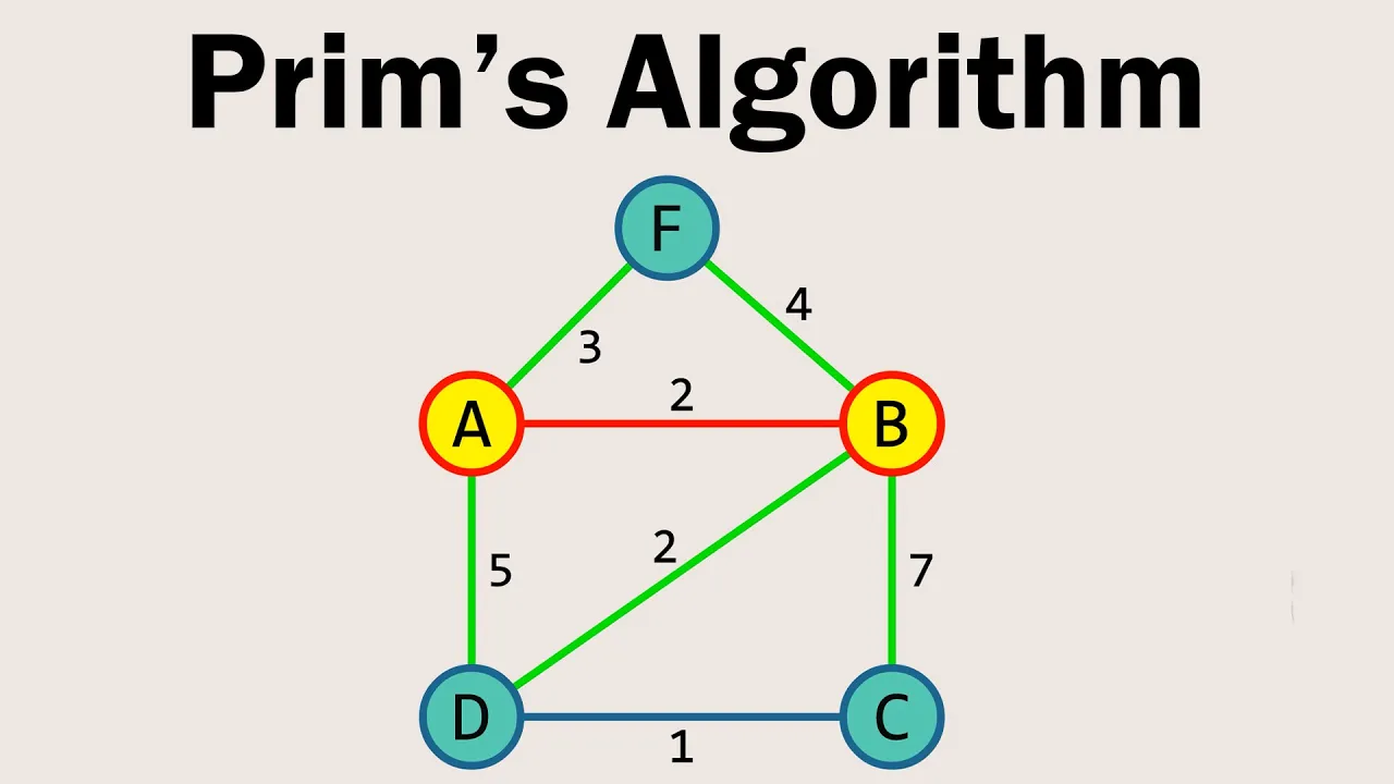
This 120-second whiteboard lesson introduces Prim's algorithm as a greedy method for building a minimum spanning tree. After defining an MST as a minimum-weight connected acyclic spanning subgraph, the presenter runs the algorithm on a 7-vertex weighted graph with vertices A through G. The Visited set starts empty, vertex A is chosen arbitrarily, and the algorithm repeatedly adds the cheapest edge crossing from visited to unvisited vertices. The worked example selects A-B, A-C, C-E, A-D, C-F, and F-G, explicitly rejecting B-E because both endpoints are already in the tree. The final MST has total edge weight 24. The clip closes by noting that Prim's time complexity depends on implementation: O(V2) with adjacency matrix searching and O(VlogV+ElogV) with a binary heap plus adjacency list.
This 16-second clip is the ending portion of a short lesson on Prim's algorithm. It first shows a handwritten summary of two running-time bounds: O(V2) for adjacency-matrix searching and O(VlogV+ElogV) for a binary heap with adjacency lists. The video then switches to a typed pseudocode page for procedure prim(G,w), displaying the input/output specification, initialization of cost and prev, construction of a priority queue H, and the main loop that extracts a minimum-cost vertex and relaxes incident edges with decreasekey. The narration says the shown algorithm is fairly easy to implement and ends by hoping the viewer understood Prim's algorithm.
Use the learning inspector for key ideas and moments, or open the reading tabs for the complete notes.
Generated from the video's visuals and explanation; not verbatim speech.
The clip opens by naming the topic: Prim's algorithm. The board pairs the title with "Minimum Spanning Tree (MST)", and the narration states that the algorithm produces a minimum-weight connected graph with no cycles. This establishes both the method and the target object before any computation begins.
A weighted example graph with vertices A through G is shown, along with the initial state Visited = { }. The narrator explains that this visited collection records which nodes have already been touched, so the viewer sees the algorithm's bookkeeping structure before the first choice is made.
The next board simplifies the initialization to "Prim's = Pick a node". The narration then applies that rule by choosing A as the arbitrary starting vertex and adding it to Visited, turning the abstract first step into a concrete example state.
From A, the algorithm examines all incident edges and selects the cheapest one leading to an unvisited vertex. The chosen edge is A-B with weight 2, which is marked as part of the growing tree, and Visited becomes {A,B}. This demonstrates the central greedy rule of Prim's algorithm.
With {A,B} visited, several frontier edges have the same minimum weight 3. The narrator explicitly treats this as a tie and chooses A-C, updating Visited to {A,B,C}. The example then continues in the same manner, adding C-E with weight 1 and A-D with weight 3 as the tree expands.
At a later stage, edge B-E has weight 3 and looks attractive, but both endpoints are already in the MST. The video uses this moment to clarify the eligibility condition: only edges crossing from visited to unvisited vertices may be taken. Therefore B-E is skipped and C-F with weight 6 is selected instead.
Once only G remains unvisited, the algorithm attaches it through F-G with weight 9. The final red subgraph spans all seven vertices and contains six edges, matching the tree requirement. The narration then adds a theoretical note: if all edge weights are distinct, the MST is unique.
The completed edge set is used to compute the objective value. The board writes the sum of the selected weights, 2+3+3+1+6+9, and evaluates it to 24, showing how the total cost of the MST is read directly from the chosen edges.
The lesson closes by shifting from the worked example to asymptotic cost. A new page lists two implementation-dependent bounds for Prim's algorithm: O(V2) for adjacency matrix searching and O(VlogV+ElogV) for a binary heap with adjacency list, while the narrator begins to explain that the running time depends on the data structures used.
The opening visual is a handwritten board titled Time Complexity. It compares two implementation choices for Prim's algorithm. The first line pairs Adjacency Matrix, Searching with O(V2), meaning that if the graph is searched through an adjacency matrix, the stated running time is quadratic in the number of vertices V.
The second line pairs Binary Heap and Adjacency List with O(VlogV+ElogV). Here E denotes the number of edges, so the bound reflects heap operations together with adjacency-list edge scans.
The video then cuts to a typed pseudocode page headed procedure prim(G,w). The input is explicitly a connected undirected graph G=(V,E) with edge weights we, and the output is a minimum spanning tree encoded by the array prev.
The algorithm begins by initializing every vertex u∈V with cost(u)=∞ and prev(u)=nil. This records that no vertex is yet attached to the growing tree. One arbitrary starting vertex u0 is then chosen and assigned cost(u0)=0 so that it becomes the first extracted vertex.
Next, the line H=makequeue(V) creates a priority queue containing all vertices, keyed by their current cost values. The narration over this page says the algorithm shown is fairly easy to implement.
The main loop runs while H is not empty. Each iteration removes v=deletemin(H), the currently cheapest frontier vertex. For every incident edge {v,z}∈E, the code checks whether cost(z)>w(v,z).
If that inequality holds, the algorithm improves z by setting cost(z)=w(v,z) and prev(z)=v, then calls decreasekey(H,z). In other words, the tree is grown by repeatedly selecting the minimum-cost available vertex and relaxing edges out of it.
The clip closes with the speaker saying, "And that's it," followed by a brief concluding remark that the video hopefully gave a good understanding of Prim's algorithm. No proof of correctness is shown in this excerpt; the emphasis is on the final complexity summary and the readable pseudocode structure.
Knowledge cards
01
Prim's algorithm produces an MST
Prim's algorithm is introduced as a greedy procedure for constructing a minimum spanning tree. The board directly links the algorithm name to "Minimum Spanning Tree (MST)", and the narration defines the MST as a minimum-weight connected graph with no cycles.
02
Definition of a minimum spanning tree
An MST is a spanning subgraph that connects all vertices, contains no cycles, and has minimum possible total edge weight. This definition is stated verbally near the beginning and serves as the target object of the whole example.
03
Initialize a Visited set
Before running the algorithm, the example creates an empty collection labeled Visited = { }. Its purpose is to record which vertices have already been incorporated into the partial tree, so future edge choices can be restricted to those crossing from visited to unvisited vertices.
04
Start from an arbitrary vertex
The first operational step is to choose any starting node. In the example, vertex A is selected and immediately added to Visited, producing Visited = {A}. This initializes the tree fragment from which the greedy expansion proceeds.
05
Greedy rule: choose the cheapest crossing edge
At each step, inspect edges from the current visited set to unvisited vertices and select the one of minimum weight. The example first chooses A-B with weight 2, then continues by adding the cheapest admissible edge at each subsequent stage.
06
Ties may be broken arbitrarily
When multiple candidate edges share the same minimum weight, any one of them may be chosen. The narrator demonstrates this when three frontier edges all have weight 3 and selects A-C as the next addition.
07
Do not add edges internal to the visited set
Even if an edge has very small weight, it must be rejected when both endpoints are already in the MST. The example explicitly skips B-E for this reason and instead adds C-F, preserving the acyclic tree structure.
08
Termination when all vertices are visited
The algorithm stops once every vertex belongs to the tree. In the example, the last unvisited vertex G is attached through F-G, leaving a connected acyclic spanning tree on all seven vertices.
09
Distinct weights imply a unique MST
The clip states that if all edge weights are distinct, then the minimum spanning tree is unique. This is presented as a theoretical note after the worked construction, not as a proved theorem within the excerpt.
10
Total MST weight is the sum of selected edge weights
After the MST edges are identified, their weights are added to obtain the objective value. The example computes 2+3+3+1+6+9=24 from the six chosen edges.
2+3+3+1+6+9=24
11
Time complexity depends on implementation
The closing board compares two standard implementations of Prim's algorithm. Using an adjacency matrix with searching gives O(V2), while using a binary heap together with an adjacency list gives O(VlogV+ElogV).
O(V2)andO(VlogV+ElogV)
12
Prim time complexity with adjacency matrix searching
The handwritten slide states that using adjacency matrix searching gives running time O(V2), where V is the number of vertices.
O(V2)
13
Prim time complexity with binary heap and adjacency list
The same slide states that using a binary heap together with adjacency lists gives running time O(VlogV+ElogV), where V is the number of vertices and E is the number of edges.
O(VlogV+ElogV)
14
Input and output of the displayed Prim procedure
The typed pseudocode defines procedure prim(G,w) for a connected undirected graph G=(V,E) with edge weights we. Its output is a minimum spanning tree represented by the array prev.
15
Initialization of Prim's algorithm
Every vertex starts with cost(u)=∞ and prev(u)=nil. An arbitrary initial vertex u0 is chosen and set to cost(u0)=0, then all vertices are inserted into a priority queue H keyed by cost.
16
Main loop and relaxation rule
While H is not empty, extract v=deletemin(H). For each edge {v,z}∈E, if cost(z)>w(v,z), update cost(z)=w(v,z), set prev(z)=v, and call decreasekey(H,z).
Detailed learning notes
Explore conditions, steps and evidence. Supplementary explanations are labeled separately from content shown in the video.
Symbols · 20
Prim's Algorithm
Clear evidence
Shown in the video
Evidence
Caption evidence
Observation
Handwritten title "Prim's Algorithm" is shown on the whiteboard.
Audio
Observation
The narrator says, "This video will show you the correct way to run Prim's algorithm on a graph."
Symbol
Prim's Algorithm
Meaning
Name of the greedy minimum spanning tree algorithm demonstrated in the clip.
Domain
Graph theory / discrete mathematics
MST
Clear evidence
Shown in the video
Evidence
Caption evidence
Observation
Below the title, the board shows "Minimum Spanning Tree (MST)" with a downward arrow from "Prim's Algorithm".
Audio
Observation
The narrator says, "Prim's algorithm results in a minimum spanning tree, a minimum weight connected graph with no cycles."
Symbol
MST
Meaning
Abbreviation for Minimum Spanning Tree, the output object produced by Prim's algorithm.
Domain
Graph theory
Visited
Clear evidence
Shown in the video
Evidence
Caption evidence
Observation
At the bottom of the graph page, the board first shows "Visited = { }" and later updates it as nodes are added.
Audio
Observation
The narrator says, "To start, create an empty list called visited. We will use this list to keep track of nodes that we have touched."
Symbol
Visited
Meaning
A tracking set/list of vertices already included in the growing minimum spanning tree.
Domain
Algorithm state in graph traversal
A, B, C, D, E, F, G
Clear evidence
Shown in the video
Evidence
Diagram
Observation
The hand-drawn graph contains seven circular nodes labeled A, B, C, D, E, F, and G.
Audio
Observation
The narrator refers to specific vertices such as A, B, C, F, and G while running the algorithm.
Symbol
A, B, C, D, E, F, G
Meaning
Vertex labels of the example weighted graph used to demonstrate Prim's algorithm.
Domain
Vertices of the example graph
Edge weights
Clear evidence
Shown in the video
Evidence
Diagram
Observation
Edges in the example graph are labeled with numeric weights including 1, 2, 3, 4, 5, 6, 7, 8, and 9.
Audio
Observation
The narrator repeatedly chooses edges by comparing their weights, e.g. "choose the smallest edge" and "edge BE with a weight of 3".
Symbol
Edge weights
Meaning
Numeric costs assigned to edges; Prim's algorithm selects the minimum-weight edge crossing from visited to unvisited vertices.
Domain
Weighted undirected graph
Total Edge Weight
Clear evidence
Shown in the video
Evidence
Caption evidence
Observation
The board writes "Total Edge Weight = 2+3+3+1+6+9=24".
Audio
Observation
The narrator says, "You can add the edge weights to get the minimum spanning tree's total edge weight."
Symbol
Total Edge Weight
Meaning
Sum of the weights of all edges selected into the MST.
Domain
Objective value of the minimum spanning tree
V
Clear evidence
Shown in the video
Evidence
Caption evidence
Observation
On the time-complexity page, the board writes O(V2) and O(VlogV+ElogV).
Audio
Observation
The narrator begins, "The time complexity depends on the data structures," indicating the formulas concern implementation-dependent running time.
Uncertainties
The clip ends before the narrator explains what V and E stand for verbally.
Symbol
V
Meaning
Number of vertices in the graph, used in the displayed time-complexity expressions.
Domain
Graph size parameter
E
Clear evidence
Shown in the video
Evidence
Caption evidence
Observation
The second complexity formula on the board is written as O(VlogV+ElogV).
Audio
Observation
The narrator introduces the topic of time complexity just before the clip ends.
Uncertainties
The clip ends before the narrator explicitly defines E in speech.
Symbol
E
Meaning
Number of edges in the graph, used in the displayed time-complexity expression.
Domain
Graph size parameter
V
Clear evidence
Shown in the video
Evidence
Formula
Observation
In the handwritten slide, V appears inside O(V2) and O(VlogV+ElogV).
Symbol
V
Meaning
Number of vertices in the graph.
Domain
Positive integer.
E
Clear evidence
Shown in the video
Evidence
Formula
Observation
In the handwritten slide, E appears inside O(VlogV+ElogV).
Symbol
E
Meaning
Number of edges in the graph.
Domain
Nonnegative integer.
G
Clear evidence
Shown in the video
Evidence
Formula
Observation
The typed pseudocode header reads procedure prim(G,w).
Symbol
G
Meaning
Input graph to Prim's algorithm.
Domain
Connected undirected graph G=(V,E).
w
Clear evidence
Shown in the video
Evidence
Formula
Observation
The typed pseudocode header reads procedure prim(G,w), and the input line mentions edge weights we.
Symbol
w
Meaning
Edge-weight function.
Domain
Assigns a weight we to each edge e.
Knowledge points · 15
Purpose of Prim's algorithm
Clear evidence
Shown in the video
Evidence
Caption evidence
Observation
Title card reads "Prim's Algorithm" with an arrow to "Minimum Spanning Tree (MST)".
Audio
Observation
Narrator states that the video shows how to run Prim's algorithm and that it results in a minimum spanning tree.
Definition
Explanation
Prim's algorithm is presented as a method for constructing a minimum spanning tree from a weighted graph. The board links the algorithm directly to the MST concept, and the narration defines the MST as a minimum-weight connected graph with no cycles.
Formula
Conditions
Applies to a weighted graph.
The desired output is a spanning tree of minimum total weight.
Prerequisites
Definition of a minimum spanning tree
Definition of a minimum spanning tree
Clear evidence
Shown in the video
Evidence
Caption evidence
Observation
The board writes "Minimum Spanning Tree (MST)" under the title.
Audio
Observation
Narrator says, "a minimum spanning tree, a minimum weight connected graph with no cycles."
Definition
Explanation
The clip defines an MST as a connected acyclic subgraph that spans the vertices and has minimum total edge weight. This is the target structure produced by Prim's algorithm.
Formula
Conditions
The graph must be connected for a spanning tree to exist.
The MST minimizes the sum of selected edge weights.
The MST contains no cycles.
Role of the Visited list/set
Clear evidence
Shown in the video
Evidence
Caption evidence
Observation
The graph page shows "Visited = { }" at the bottom.
Audio
Observation
Narrator says to create an empty list called visited to keep track of nodes that have been touched.
Method
Explanation
Prim's algorithm maintains a collection of already included vertices. In the example, this is written as a set-like object "Visited" and updated after each chosen vertex is incorporated into the growing tree.
Formula
Conditions
Used during execution of Prim's algorithm.
Initially empty before the first vertex is chosen.
Prerequisites
Purpose of Prim's algorithm
Starting step of Prim's algorithm
Clear evidence
Shown in the video
Evidence
Caption evidence
Observation
A separate board page reads "Prim's = Pick a node".
Audio
Observation
Narrator says, "The next step is to pick an arbitrary node. We will start the algorithm from this node. Let's start with A in our graph. First, add A to the visited list."
Method
Explanation
The algorithm begins by choosing any starting vertex. In the worked example, vertex A is selected and immediately inserted into the Visited set, establishing the initial tree fragment.
Formula
Conditions
The starting vertex may be chosen arbitrarily.
After selection, the starting vertex is marked visited.
Prerequisites
Role of the Visited list/set
Greedy selection rule in Prim's algorithm
Clear evidence
Shown in the video
Evidence
Audio
Observation
Narrator says, "Next, examine all vertices reachable from A... Prim's is a greedy algorithm, so we're going to choose the smallest edge that connects to an unvisited node, in this case, A to B."
Diagram
Observation
Edges from A are highlighted, and the edge A-B with weight 2 is circled and then colored red as part of the MST.
Method
Explanation
At each iteration, the algorithm inspects edges incident to the current visited set and chooses the minimum-weight edge that leads to a vertex not yet visited. The chosen edge and its new endpoint are then added to the MST.
Formula
Conditions
Consider only edges crossing from visited vertices to unvisited vertices.
Choose the edge of minimum weight among those candidates.
Add both the edge and the newly reached vertex to the tree.
Prerequisites
Starting step of Prim's algorithm
Role of the Visited list/set
Tie handling when several minimum edges have equal weight
Clear evidence
Shown in the video
Evidence
Audio
Observation
Narrator says, "Three edges all have a weight of three. Pick one of these. I've chosen to add AC."
Diagram
Observation
From the visited set {A,B}, multiple candidate edges of weight 3 are visible, and A-C is selected next.
Method
Explanation
When more than one candidate edge attains the same minimum weight, the algorithm may choose any one of them. In the example, after {A,B} are visited, several weight-3 edges are available and the presenter selects A-C.
Formula
Conditions
Occurs when multiple crossing edges share the minimum weight.
Any tied edge may be chosen without violating the greedy rule.
Prerequisites
Greedy selection rule in Prim's algorithm
Reject edges whose endpoints are both already visited
Clear evidence
Shown in the video
Evidence
Audio
Observation
Narrator says, "Notice at this point, the edge BE with a weight of 3 is the smallest edge. But both vertices are already in the MST, so we do not pick it. Instead, we will choose to add F to the MST."
Diagram
Observation
Edge B-E remains blue/unselected while the algorithm instead selects C-F with weight 6.
Method
Explanation
Prim's algorithm only accepts edges that connect the visited portion of the tree to an unvisited vertex. Even if an edge has small weight, it is ignored when both endpoints are already in the MST, because adding it would create a cycle.
Formula
Conditions
Candidate edge must cross between visited and unvisited vertices.
Edges internal to the visited set are discarded.
Prerequisites
Greedy selection rule in Prim's algorithm
Definition of a minimum spanning tree
Termination condition and completed MST
Clear evidence
Shown in the video
Evidence
Audio
Observation
Narrator says, "The only unvisited node remaining is G, so we add this to the minimum spanning tree. All the nodes are now connected in a tree."
Diagram
Observation
The final red MST includes all seven vertices A through G and six selected edges.
Method
Explanation
The process stops once every vertex has been visited and included in the tree. In the example, the last unvisited vertex G is attached through edge F-G, yielding a connected acyclic spanning tree over all vertices.
Formula
Conditions
Continue until all vertices are in the Visited set.
For a connected graph with n vertices, the MST contains n-1 edges.
Narrator says, "You can add the edge weights to get the minimum spanning tree's total edge weight."
Formula
Explanation
After the MST edges are selected, the total cost is obtained by summing their weights. The example computes the total from the six chosen edges and obtains 24.
Formula
2+3+3+1+6+9=24
Conditions
Apply after the MST edge set has been determined.
Sum only the weights of edges included in the MST.
Prerequisites
Termination condition and completed MST
Implementation-dependent time complexity of Prim's algorithm
Clear evidence
Shown in the video
Evidence
Caption evidence
Observation
Board heading "Time Complexity" lists "Adjacency Matrix, Searching -> O(V2)" and "Binary Heap and Adjacency List -> O(VlogV+ElogV)".
Audio
Observation
Narrator says, "The time complexity depends on the data structures," before the clip ends.
Uncertainties
The verbal explanation is cut off before the narrator elaborates on why each implementation gives the stated bound.
Formula
Explanation
The clip states that Prim's running time depends on the chosen data structures. Two standard implementations are shown: using an adjacency matrix with searching gives O(V2), while using a binary heap together with an adjacency list gives O(VlogV+ElogV).
Formula
O(V2)andO(VlogV+ElogV)
Conditions
First bound corresponds to adjacency-matrix search implementation.
Second bound corresponds to binary-heap plus adjacency-list implementation.
V denotes number of vertices and E denotes number of edges.
Prerequisites
Purpose of Prim's algorithm
Time complexity using adjacency matrix searching
Clear evidence
Shown in the video
Evidence
Formula
Observation
Handwritten slide title Time Complexity with line Adjacency Matrix, Searching -> O(V2).
Formula
Explanation
The slide states that when Prim's algorithm is implemented with adjacency-matrix searching, the running time is O(V2). Here V denotes the number of vertices.
Formula
O(V2)
Conditions
Implementation uses adjacency matrix searching.
V is the number of vertices.
Prerequisites
V
Time complexity using binary heap and adjacency list
Clear evidence
Shown in the video
Evidence
Formula
Observation
Handwritten slide line Binary Heap and Adjacency List -> O(VlogV+ElogV).
Formula
Explanation
The slide states that with a binary heap and adjacency list representation, the running time is O(VlogV+ElogV). Here V is the number of vertices and E is the number of edges.
Formula
O(VlogV+ElogV)
Conditions
Implementation uses a binary heap.
Graph is stored with adjacency lists.
V is the number of vertices and E is the number of edges.
Prerequisites
V
E
Claims and conditions · 5
Characterization of a minimum spanning tree
Clear evidence
Shown in the video
Evidence
Audio
Observation
Narrator defines MST as "a minimum weight connected graph with no cycles."
Caption evidence
Observation
Board labels the output as "Minimum Spanning Tree (MST)".
Proposition
Statement
A minimum spanning tree is a connected acyclic spanning subgraph of minimum total edge weight.
Hypotheses
The underlying graph is weighted.
A spanning tree exists, which requires connectivity of the graph.
Quantifiers
For the given weighted connected graph, an MST is a spanning subgraph with minimum total weight among all spanning trees.
Uniqueness of MST under distinct edge weights
Clear evidence
Shown in the video
Evidence
Audio
Observation
Narrator says, "Note that if edge weights are distinct, this minimum spanning tree will be unique."
Uncertainties
The clip states the result but does not prove it.
Proposition
Statement
If all edge weights in the graph are distinct, then the minimum spanning tree is unique.
Hypotheses
The graph is weighted.
All edge weights are pairwise distinct.
Quantifiers
For any weighted graph whose edge weights are all different, there is exactly one minimum spanning tree.
Prim's algorithm uses a greedy local choice
Clear evidence
Shown in the video
Evidence
Audio
Observation
Narrator says, "Prim's is a greedy algorithm, so we're going to choose the smallest edge that connects to an unvisited node."
Proposition
Statement
Prim's algorithm proceeds by greedily selecting the minimum-weight edge that connects the current visited set to an unvisited vertex.
Hypotheses
A starting vertex has been chosen.
A visited set is maintained.
Edge weights are comparable.
Quantifiers
At each iteration before completion, the algorithm chooses a locally minimum crossing edge.
Running time depends on implementation
Clear evidence
Shown in the video
Evidence
Audio
Observation
Narrator says, "The time complexity depends on the data structures," while introducing the complexity page.
Caption evidence
Observation
Two different bounds are written for two different implementations.
Uncertainties
The spoken explanation is truncated before further detail is given.
Proposition
Statement
The time complexity of Prim's algorithm depends on the data structures used to represent and search the graph.
Hypotheses
The graph is represented in some concrete data structure.
The algorithm is implemented using a corresponding search/update mechanism.
Quantifiers
Across implementations of Prim's algorithm, asymptotic running time varies with the chosen representation and priority-structure support.
Ease of implementing the shown algorithm
Clear evidence
Shown in the video
Evidence
Audio
Observation
Speaker says: "The algorithm shown here is fairly easy to implement."
Uncertainties
This is an evaluative statement rather than a formal theorem.
Proposition
Statement
The algorithm shown on screen is fairly easy to implement.
Hypotheses
The speaker is referring to the displayed Prim pseudocode.
Quantifiers
No formal quantifier is stated.
Derivations and proofs · 3
Step-by-step execution of Prim's algorithm on the example graph
Clear evidence
Shown in the video
Evidence
Audio
Observation
The narrator walks through the algorithm step by step on the example graph.
Diagram
Observation
The board updates Visited and colors selected MST edges in red as the algorithm proceeds.
Visual argument
Steps
Expression
Explanation
Begin with an empty Visited set, written as Visited = { }.
Justification
Initialization step stated by the narrator.
Shown in the video
Expression
Explanation
Pick an arbitrary starting vertex; the example chooses A and updates Visited = {A}.
Justification
The narrator says to pick an arbitrary node and then starts with A.
Shown in the video
Expression
Explanation
Examine edges incident to A and choose the minimum-weight edge to an unvisited vertex, namely A-B with weight 2; update Visited = {A,B}.
Justification
This is the greedy rule described in the narration and shown by circling A-B.
Shown in the video
Expression
Explanation
From the visited set {A,B}, compare crossing edges; several have weight 3, and the presenter chooses A-C, updating Visited = {A,B,C}.
Justification
The narrator explicitly notes the tie among weight-3 edges and says, "I've chosen to add AC."
Shown in the video
Expression
Explanation
Continue the same rule and select C-E with weight 1, updating Visited = {A,B,C,E}.
Justification
The board shows C-E circled and then colored red as the next minimum crossing edge.
Shown in the video
Expression
Explanation
Select A-D with weight 3, updating Visited = {A,B,C,E,D}.
Justification
The diagram highlights A-D next and the narration instructs to continue picking the smallest edge to an unvisited node.
Shown in the video
Expression
Explanation
Although B-E has weight 3, it is not chosen because both B and E are already visited; instead choose C-F with weight 6, updating Visited = {A,B,C,D,E,F}.
Justification
The narrator explicitly rejects B-E for having both endpoints in the MST and then adds F.
Shown in the video
Expression
Explanation
The only remaining unvisited vertex is G, so add F-G with weight 9 and obtain the full MST over all seven vertices.
Justification
The narrator states that G is the only unvisited node remaining and then declares all nodes connected in a tree.
Shown in the video
Expression
2+3+3+1+6+9=24
Explanation
Sum the weights of the six selected MST edges to compute the total edge weight.
Justification
The board writes the arithmetic and the narrator explains that the MST total is found by adding edge weights.
Shown in the video
Conclusion
The example yields the MST edge set {A-B, A-C, C-E, A-D, C-F, F-G} with total weight 24.
Why an already-internal minimum edge is skipped
Clear evidence
Shown in the video
Evidence
Audio
Observation
Narrator says edge BE is smallest but both vertices are already in the MST, so it is not picked.
Diagram
Observation
B-E remains unselected while another crossing edge is chosen instead.
Intuitive argument
Steps
Expression
Explanation
Identify the smallest visible edge among candidates, here B-E with weight 3.
Justification
The narrator points out that B-E is the smallest edge at that moment.
Shown in the video
Expression
Explanation
Check whether the edge connects a visited vertex to an unvisited vertex.
Justification
Prim's rule only accepts crossing edges from the current tree to outside vertices.
Derived from the video
Expression
Explanation
Since both B and E are already in the MST, reject B-E.
Justification
The narrator explicitly says both vertices are already in the MST, so the edge is not picked.
Shown in the video
Expression
Explanation
Choose the next valid minimum crossing edge, C-F with weight 6.
Justification
The algorithm continues by selecting the smallest admissible edge to an unvisited node.
Shown in the video
Conclusion
Edges internal to the visited set are ignored because accepting them would violate the tree/no-cycle requirement of an MST.
Algorithmic flow of the displayed Prim procedure
Clear evidence
Shown in the video
Evidence
Formula
Observation
Full typed pseudocode for procedure prim(G,w) is visible from initialization through the while-loop and decreasekey update.
Uncertainties
The clip does not prove correctness; it only displays the algorithmic steps.
Intuitive argument
Steps
Expression
forallu∈V:cost(u)=∞,prev(u)=nil
Explanation
Initialize every vertex with infinite cost and no predecessor.
Justification
Displayed pseudocode initialization.
Shown in the video
Expression
Pickanyinitialnodeu0;cost(u0)=0
Explanation
Choose one starting vertex and give it zero cost so it will be selected first.
Justification
Displayed pseudocode initialization.
Shown in the video
Expression
H=makequeue(V)
Explanation
Place all vertices into a priority queue keyed by cost-values.
Justification
Displayed pseudocode line with parenthetical note priority queue, using cost-values as keys.
Shown in the video
Expression
whileHisnotempty:v=deletemin(H)
Explanation
Repeatedly remove the currently cheapest unreached vertex from the queue.
For each neighbor z of v, improve z's connection to the tree if edge {v,z} is cheaper than its current cost, then update the queue key.
Justification
Displayed relaxation block.
Shown in the video
Conclusion
The procedure grows a spanning tree by always extracting the minimum-cost frontier vertex and relaxing incident edges, with the final tree encoded in prev.
Worked examples · 1
Worked example: Prim's algorithm on a 7-vertex weighted graph
Clear evidence
Shown in the video
Evidence
Diagram
Observation
A weighted graph with vertices A through G and numeric edge weights is drawn and processed step by step.
Audio
Observation
The narrator runs Prim's algorithm on this exact graph and computes the final total weight.
Problem
Run Prim's algorithm on the displayed weighted graph with vertices A, B, C, D, E, F, G and find its minimum spanning tree and total edge weight.
Start by choosing an arbitrary node; the example chooses A.
Goal
Construct the MST using Prim's greedy rule and compute the total edge weight.
Steps
Expression
Explanation
Initialize Visited = { }.
Justification
Stated initialization step of the algorithm.
Shown in the video
Expression
Explanation
Choose A as the start vertex and set Visited = {A}.
Justification
The narrator says to pick an arbitrary node and starts with A.
Shown in the video
Expression
Explanation
Select A-B (weight 2) as the minimum edge from A to an unvisited vertex; set Visited = {A,B}.
Justification
Direct application of the greedy crossing-edge rule.
Shown in the video
Expression
Explanation
Among tied minimum crossing edges of weight 3, choose A-C; set Visited = {A,B,C}.
Justification
The narrator notes the tie and explicitly chooses AC.
Shown in the video
Expression
Explanation
Select C-E (weight 1); set Visited = {A,B,C,E}.
Justification
It is the smallest edge from the visited set to an unvisited vertex at that stage.
Shown in the video
Expression
Explanation
Select A-D (weight 3); set Visited = {A,B,C,E,D}.
Justification
Continuation of the same greedy rule as shown on the board.
Shown in the video
Expression
Explanation
Skip B-E because both endpoints are already visited; select C-F (weight 6); set Visited = {A,B,C,D,E,F}.
Justification
The narrator explicitly rejects B-E and then adds F via C-F.
Shown in the video
Expression
Explanation
Select F-G (weight 9) as the last remaining unvisited vertex is G.
Justification
The narrator states that G is the only unvisited node left.
Shown in the video
Expression
2+3+3+1+6+9=24
Explanation
Add the weights of the six MST edges to obtain the total cost.
Justification
The board displays the arithmetic and the narrator explains the summation.
Shown in the video
Answer
The MST consists of edges A-B, A-C, C-E, A-D, C-F, and F-G, with total edge weight 24.
Verification
The resulting subgraph connects all seven vertices, contains exactly six edges, and has no cycles; the displayed sum of selected edge weights is 24.
Visual events · 10
Title card linking algorithm to output object
Clear evidence
Shown in the video
Evidence
Caption evidence
Observation
The opening board shows "Prim's Algorithm" and then adds a downward arrow to "Minimum Spanning Tree (MST)".
Objects
Text "Prim's Algorithm"
Downward arrow
Text "Minimum Spanning Tree (MST)"
Changes
The board first presents the algorithm name.
An arrow is added to indicate the algorithm produces an MST.
Invariants
The relationship shown is conceptual rather than computational.
No graph is yet being processed in this interval.
Interpretation
The visual establishes that Prim's algorithm is being introduced as a method for obtaining a minimum spanning tree.
Initial example graph and empty visited set
Clear evidence
Shown in the video
Evidence
Diagram
Observation
A hand-drawn weighted graph with vertices A through G appears, with "Visited = { }" written below.
Objects
Seven labeled vertices A-G
Weighted edges
Text "Visited = { }"
Changes
The example graph is introduced.
The algorithm state is initialized with an empty visited collection.
Invariants
The underlying graph structure and edge weights remain fixed throughout the worked example.
No MST edges are selected yet.
Interpretation
This frame sets up the input instance before any greedy choices are made.
Simplified statement of the first algorithmic action
Clear evidence
Shown in the video
Evidence
Caption evidence
Observation
A separate board page reads "Prim's = Pick a node".
Objects
Text "Prim's = Pick a node"
Changes
The video temporarily leaves the graph to emphasize the initialization rule.
Invariants
No vertex has yet been permanently added on this slide itself.
The message summarizes the next operational step.
Interpretation
The visual compresses the start of Prim's algorithm to the idea of choosing an initial vertex.
First greedy expansion from vertex A
Clear evidence
Shown in the video
Evidence
Diagram
Observation
Edges incident to A are emphasized, and A-B is circled and then colored red.
Audio
Observation
Narrator says to examine all vertices reachable from A and choose the smallest edge to an unvisited node.
Objects
Vertex A
Edges from A
Edge A-B
Visited set text
Changes
Visited changes from { } to {A}, then to {A,B}.
Edge A-B is marked as part of the MST.
Invariants
The rest of the graph topology is unchanged.
Only edges crossing from visited to unvisited vertices are relevant.
Interpretation
The animation/diagram demonstrates the core Prim step: inspect frontier edges and take the cheapest one leading outward.
Tie among minimum-weight frontier edges
Clear evidence
Shown in the video
Evidence
Diagram
Observation
Multiple candidate edges of weight 3 are visible from the visited set, and A-C is circled and selected.
Audio
Observation
Narrator says three edges all have weight 3 and chooses AC.
Objects
Visited set {A,B}
Candidate edges of weight 3
Edge A-C
Changes
Visited expands from {A,B} to {A,B,C}.
One tied minimum edge is selected arbitrarily.
Invariants
All tied edges have equal weight.
The algorithm remains valid regardless of which tied edge is chosen.
Interpretation
The visual illustrates that Prim's greedy rule may encounter ties and still proceed by selecting any minimum crossing edge.
Rejection of an internal edge and continuation of the frontier rule
Clear evidence
Shown in the video
Evidence
Diagram
Observation
Edge B-E is visible with weight 3 but remains unselected, while C-F is chosen next.
Audio
Observation
Narrator explicitly says B-E is not picked because both vertices are already in the MST.
Objects
Edge B-E
Edge C-F
Visited set before and after addition of F
Changes
The algorithm ignores B-E despite its low weight.
Visited expands by adding F through C-F.
Invariants
Accepted edges must always cross from visited to unvisited vertices.
The visited set only grows; it never shrinks.
Interpretation
This event visually clarifies a common misconception: the globally smallest adjacent edge is not always eligible if it stays inside the current tree.
Completed MST and objective-value calculation
Clear evidence
Shown in the video
Evidence
Diagram
Observation
All seven vertices are circled in red and the selected MST edges are shown in red.
Caption evidence
Observation
The board writes "Total Edge Weight = 2+3+3+1+6+9=24".
Objects
Red-highlighted MST edges
All vertices A-G
Arithmetic line for total weight
Changes
The algorithm reaches termination with all vertices visited.
The total weight is computed from the selected edges.
Invariants
The final structure is a tree spanning all vertices.
The non-selected edges are omitted from the MST.
Interpretation
The closing graph view confirms the output of Prim's algorithm and translates the edge set into its numerical cost.
Transition from worked example to asymptotic analysis
Clear evidence
Shown in the video
Evidence
Caption evidence
Observation
A new page titled "Time Complexity" lists two implementation-dependent bounds.
Uncertainties
The narrator's explanation is cut off before elaboration.
Objects
Heading "Time Complexity"
Text "Adjacency Matrix, Searching -> O(V2)"
Text "Binary Heap and Adjacency List -> O(VlogV+ElogV)"
Changes
The video shifts from concrete graph execution to general algorithm analysis.
Invariants
The bounds are presented as properties of implementations, not of a single graph instance.
Interpretation
The board summarizes that Prim's efficiency depends on how the graph and priority operations are implemented.
Handwritten time-complexity summary
Clear evidence
Shown in the video
Evidence
Diagram
Observation
Static handwritten page titled Time Complexity with two implementation lines and arrows to asymptotic bounds.
Objects
Title Time Complexity
Line Adjacency Matrix, Searching
Arrow
Expression O(V2)
Line Binary Heap and Adjacency List
Arrow
Expression O(VlogV+ElogV)
Changes
At about 3.5 seconds the handwritten page gives way to a typed pseudocode page.
Invariants
During the first 3.5 seconds the slide content remains static.
The two complexity statements stay paired with their implementation labels.
Interpretation
The visual introduces implementation-dependent running times before showing the algorithm itself.
Typed Prim pseudocode display
Clear evidence
Shown in the video
Evidence
Diagram
Observation
Static typed page headed procedure prim(G,w) with input/output lines, initialization, priority queue creation, and nested loops.
Objects
Header procedure prim(G,w)
Input line
Output line
Initialization block
H = makequeue(V)
while-loop
for each {v,z} ∈E
if cost(z) > w(v,z)
decreasekey(H,z)
Source URL at bottom right
Changes
Around 3.5 seconds the previous handwritten slide is replaced by this typed page.
After the transition the page remains static until the end of the clip.
Invariants
The pseudocode text does not animate or highlight individual lines.
The source citation remains visible at the bottom right.
Interpretation
The second visual presents the full algorithm in pseudocode form while the narration comments on ease of implementation and concludes the lesson.
Misconceptions · 2
Misconception: choose the smallest edge regardless of endpoint status
Clear evidence
Shown in the video
Evidence
Audio
Observation
Narrator says the edge BE with weight 3 is the smallest edge, but both vertices are already in the MST, so it is not picked.
Diagram
Observation
B-E is left unselected while another crossing edge is chosen.
Misconception
One might think Prim's algorithm should always take the smallest nearby edge, even if both endpoints are already in the tree.
Clarification
Prim's rule only accepts the smallest edge connecting the visited set to an unvisited vertex. Edges internal to the visited set are rejected because they would create a cycle.
Misconception: the MST is always unique
Clear evidence
Shown in the video
Evidence
Audio
Observation
Narrator says, "Note that if edge weights are distinct, this minimum spanning tree will be unique."
Uncertainties
The clip does not discuss what happens when weights are not distinct, beyond implying non-uniqueness may occur.
Misconception
A learner may infer from the example that every graph has exactly one MST.
Clarification
The video states uniqueness only under the additional condition that all edge weights are distinct. Without that condition, multiple MSTs can exist.
Concept relations · 10
Purpose of Prim's algorithm → Definition of a minimum spanning tree
Clear evidence
Shown in the video
Evidence
Caption evidence
Observation
Arrow from "Prim's Algorithm" to "Minimum Spanning Tree (MST)".
Audio
Observation
Narrator says Prim's algorithm results in a minimum spanning tree.
Application
Explanation
Prim's algorithm is presented as a procedure whose output is a minimum spanning tree.
Role of the Visited list/set → Greedy selection rule in Prim's algorithm
Clear evidence
Shown in the video
Evidence
Audio
Observation
The visited list is introduced and then used to decide which edges connect to unvisited nodes.
Diagram
Observation
Visited is updated after each accepted vertex.
Prerequisite
Explanation
Maintaining the visited set is necessary in order to identify which edges cross from the current tree to unvisited vertices.
Greedy selection rule in Prim's algorithm → Termination condition and completed MST
Clear evidence
Shown in the video
Evidence
Audio
Observation
The narrator repeats the greedy rule until all nodes are connected in a tree.
Diagram
Observation
Each accepted crossing edge enlarges the partial MST until all vertices are included.
Proof dependency
Explanation
The termination argument depends on repeatedly applying the greedy crossing-edge rule until every vertex has been absorbed into the tree.
Reject edges whose endpoints are both already visited → Definition of a minimum spanning tree
Clear evidence
Shown in the video
Evidence
Audio
Observation
Narrator rejects B-E because both endpoints are already in the MST.
Diagram
Observation
The selected edges continue to form an acyclic connected subgraph.
Application
Explanation
Discarding internal edges is what keeps the construction consistent with the no-cycle requirement of a spanning tree.
Termination condition and completed MST → Computing the MST objective value
Clear evidence
Shown in the video
Evidence
Caption evidence
Observation
The total-weight arithmetic is written after the final red MST is shown.
Audio
Observation
Narrator says to add the edge weights to get the MST's total edge weight.
Prerequisite
Explanation
The total edge weight can be computed only after the MST edge set has been fully determined.
Purpose of Prim's algorithm → Implementation-dependent time complexity of Prim's algorithm
Clear evidence
Shown in the video
Evidence
Caption evidence
Observation
Two different bounds are listed for two different implementations.
Audio
Observation
Narrator says the time complexity depends on the data structures.
Uncertainties
The clip ends before giving a detailed derivation of either bound.
Application
Explanation
The abstract algorithm Prim's method can be implemented in multiple ways, and the chosen data structures determine its asymptotic running time.
Time complexity using adjacency matrix searching → Main relaxation loop of Prim's algorithm
Clear evidence
Shown in the video
Evidence
Formula
Observation
Adjacency Matrix, Searching is directly paired by an arrow with O(V2).
Application
Explanation
The O(V2) bound applies to the displayed Prim procedure when implemented with adjacency-matrix searching.
Time complexity using binary heap and adjacency list → Main relaxation loop of Prim's algorithm
Clear evidence
Shown in the video
Evidence
Formula
Observation
Binary Heap and Adjacency List is directly paired by an arrow with O(VlogV+ElogV).
Application
Explanation
The O(VlogV+ElogV) bound applies to the displayed Prim procedure when implemented with a binary heap and adjacency lists.
Initialization step of Prim's algorithm → Main relaxation loop of Prim's algorithm
Clear evidence
Shown in the video
Evidence
Formula
Observation
Initialization lines precede H = makequeue(V) and the while-loop in the same pseudocode block.
Prerequisite
Explanation
The main loop depends on the prior initialization of cost, prev, the seed vertex u0, and the priority queue H.
Main relaxation loop of Prim's algorithm → Problem solved by the displayed Prim procedure
Clear evidence
Shown in the video
Evidence
Formula
Observation
The procedure header and input/output lines frame the subsequent algorithm as solving the minimum spanning tree problem.
Application
Explanation
The displayed method is an implementation of Prim's algorithm for producing a minimum spanning tree from a connected undirected weighted graph.
Find an answer · 13
What is a minimum spanning tree?
Clear evidence
Shown in the video
Evidence
Audio
Observation
Narrator defines MST as a minimum weight connected graph with no cycles.
Knowledge points
Definition of a minimum spanning tree
Purpose of Prim's algorithm
How do you start Prim's algorithm on a graph?
Clear evidence
Shown in the video
Evidence
Caption evidence
Observation
Board says "Prim's = Pick a node".
Audio
Observation
Narrator says to pick an arbitrary node and start with A.
Knowledge points
Starting step of Prim's algorithm
Role of the Visited list/set
Why is edge A-B chosen first in the example?
Clear evidence
Shown in the video
Evidence
Audio
Observation
Narrator chooses the smallest edge from A to an unvisited node, A to B.
Diagram
Observation
A-B is circled and colored red.
Knowledge points
Greedy selection rule in Prim's algorithm
What should you do when several candidate edges have the same minimum weight?
Clear evidence
Shown in the video
Evidence
Audio
Observation
Narrator says three edges all have weight 3 and picks one of them.
Knowledge points
Tie handling when several minimum edges have equal weight
Why is edge B-E skipped even though it has weight 3?
Clear evidence
Shown in the video
Evidence
Audio
Observation
Narrator says B-E is not picked because both vertices are already in the MST.
Knowledge points
Reject edges whose endpoints are both already visited
Misconception: choose the smallest edge regardless of endpoint status
Is the minimum spanning tree always unique?
Clear evidence
Shown in the video
Evidence
Audio
Observation
Narrator says the MST will be unique if edge weights are distinct.
Knowledge points
Uniqueness of MST under distinct edge weights
Misconception: the MST is always unique
How do you compute the total weight of the MST after running Prim's algorithm?
Clear evidence
Shown in the video
Evidence
Caption evidence
Observation
Board shows the sum 2+3+3+1+6+9=24.
Knowledge points
Computing the MST objective value
What is the time complexity of Prim's algorithm with different data structures?
Clear evidence
Shown in the video
Evidence
Caption evidence
Observation
Board lists O(V2) and O(VlogV+ElogV) for different implementations.
Uncertainties
The spoken explanation is truncated.
Knowledge points
Implementation-dependent time complexity of Prim's algorithm
What time complexity does the video state for Prim's algorithm with adjacency matrix searching?
Clear evidence
Shown in the video
Evidence
Formula
Observation
Handwritten line Adjacency Matrix, Searching -> O(V2).
Knowledge points
Time complexity using adjacency matrix searching
What time complexity does the video state for Prim's algorithm using a binary heap and adjacency list?
Clear evidence
Shown in the video
Evidence
Formula
Observation
Handwritten line Binary Heap and Adjacency List -> O(VlogV+ElogV).
Knowledge points
Time complexity using binary heap and adjacency list
How does the displayed Prim pseudocode initialize the algorithm?
Clear evidence
Shown in the video
Evidence
Formula
Observation
Pseudocode initializes cost and prev for all vertices, then sets cost(u0)=0 and builds H.
Knowledge points
Initialization step of Prim's algorithm
When does the pseudocode call decreasekey(H,z) and what does that update accomplish?
Clear evidence
Shown in the video
Evidence
Formula
Observation
Inside the if-block the pseudocode updates cost(z), prev(z), and calls decreasekey(H,z).
Knowledge points
Main relaxation loop of Prim's algorithm
Coverage and review notes
Covered · Title card and verbal definition introduce Prim's algorithm and the MST output.
Covered · Example graph is shown and the empty Visited set is initialized.
Covered · Board states to pick a node; narration selects A as the starting vertex.
Covered · Edges from A are examined and A-B is chosen as the first MST edge.
Covered · Tied weight-3 edges are discussed; A-C is chosen, then the process continues toward C-E and A-D.
Covered · B-E is rejected because both endpoints are already visited; C-F is added instead.
Covered · G is added as the last vertex, the MST is complete, and uniqueness under distinct weights is stated.
Covered · The selected edge weights are summed to obtain total weight 24.
Covered · A new board lists implementation-dependent time complexities before the clip ends.
Covered · Handwritten slide presents two implementation-dependent time complexities for Prim's algorithm.
Covered · Typed pseudocode shows the full Prim procedure while the audio comments on ease of implementation and closes the lesson.
Covered · Final brief tail after the spoken conclusion; no additional mathematical content is introduced.
Reviewed English material v1: card/concept_card "Prim's algorithm produces an MST" starting at 0:00 — Prim's algorithm is introduced as a greedy procedure for constructing a minimum spanning tree. The board directly links the algorithm name to "Minimum Spanning Tree (MST)", and the narration defines the MST as a minimum-weight connected graph with no cycles.
When multiple candidate edges share the same minimum weight, you can pick any one of them. The choice does not affect the validity of the greedy step, though it may lead to a different MST if edge weights are not distinct.
Conditions: Multiple edges connect the visited set to unvisited nodes.; These edges have identical minimum weights.
The time complexity of Prim's algorithm depends on the data structures used. Using an adjacency matrix with searching gives O(V2), while using a binary heap with an adjacency list gives O(VlogV+ElogV), where V is the number of vertices and E is the number of edges.
Conditions: The graph is represented using specific data structures.; V denotes the number of vertices.; E denotes the number of edges.
Edge B-E is skipped because both of its endpoints (B and E) are already in the visited set (MST). Prim's algorithm only considers edges that connect a visited vertex to an unvisited vertex to avoid creating cycles.
Conditions: Both endpoints of the edge are already marked as visited.; The algorithm strictly follows the rule of adding only crossing edges.
To start Prim's algorithm, create an empty list called 'visited' to track touched nodes, then pick an arbitrary starting node and add it to the visited list.
Conditions: The graph is weighted and connected.; You have a mechanism to track visited vertices (e.g., a list or set).
To compute the total weight of the MST, sum the weights of all edges that were selected and added to the tree during the execution of Prim's algorithm.
Conditions: The MST edge set has been fully determined.; You have access to the weights of the selected edges.
Edge A-B is chosen first because Prim's algorithm is a greedy algorithm that selects the smallest edge connecting the current visited set to an unvisited node. From the starting node A, edge A-B has the minimum weight among all edges incident to A leading to unvisited nodes.
Conditions: Node A is the starting visited node.; The algorithm follows the greedy rule of picking the minimum-weight crossing edge.
A minimum spanning tree (MST) is a connected, acyclic subgraph that spans all vertices of a weighted graph and has the minimum possible total edge weight.
Conditions: The underlying graph must be weighted.; The graph must be connected for a spanning tree to exist.; The MST minimizes the sum of selected edge weights.; The MST contains no cycles.