Reviewed learning material · Video analysis · EnglishRead the full overview
This 3-minute introductory explainer defines linear regression as fitting a line (or hyperplane) to data points for prediction. It introduces the model y=mx+b (or f(x)=β1x+β0), explains the roles of slope and intercept, extends the idea to multiple input variables, and then motivates the least-squares criterion through residuals, squared errors, and the SSE loss function. The clip closes by showing gradient descent as a way to minimize SSE and by describing a 2/3 train, 1/3 test split for validation.
This 54-second clip is the ending portion of a short linear-regression explainer. It first shows a scatter plot with a yellow regression line while the narrator says the purpose is to ensure the regression performs well on data it has not seen before. It then switches to a “Performance Metrics” slide that lists four evaluation concepts for linear regression: R2, Standard Error of the Estimate, Prediction Interval, and Statistical Significance, each with a brief on-screen definition. The remainder is promotional outro material about the creator’s books and O’Reilly courses, followed by a black screen with music.
Use the learning inspector for key ideas and moments, or open the reading tabs for the complete notes.
Generated from the video's visuals and explanation; not verbatim speech.
The clip opens with a brief animated logo and the title "Linear Regression in 3 Minutes". No mathematics is presented yet; this section functions as branding and topic introduction.
The first mathematical scene shows a scatter plot of cyan points on black axes. A yellow straight line is then drawn through the cloud of points. Over this image, the narration defines linear regression as a statistical technique for modeling the relationship between an output variable and one or more input variables. The visual simplifies that definition to the familiar task of fitting a line through data so that predictions can be made on unseen inputs, provided the relationship is approximately linear.
The plot gives way to the equation y=mx+b. A highlight box marks y and labels it "Output", matching the narration that y is the dependent variable. The equation is then rewritten as f(x)=mx+b, and the highlight shifts to x with the label "Input", establishing that x is the independent variable. This segment connects symbolic notation to the earlier scatter-plot picture: the line is not just a drawing, but the graph of a function of the input.
The same model is restated in statistical notation as y=β1x+β0, and later as f(x)=β1x+β0. The narration explains that β1 corresponds to the slope and β0 to the intercept, also called the bias in machine learning. The animation makes the distinction concrete: when the slope term is emphasized, the line pivots; when the intercept term is emphasized, the whole line shifts vertically. The segment ends by stating that these two coefficients are the quantities linear regression solves for, and a numeric example f(x)=1.93939x+4.73333 appears.
The equation expands step by step from one input to several inputs: y=β2x2+β1x1+β0, then y=β3x3+β2x2+β1x1+β0, and onward to y=β5x5+β4x4+β3x3+β2x2+β1x1+β0. The narration says each new beta acts as a slope for its corresponding variable. The visual then jumps to three dimensions, where a cyan grid plane passes through a scattered point cloud. This illustrates the claim that in higher dimensions the fitted object is a hyperplane rather than a line.
Returning to the 2D scatter plot, the video asks how to choose the best line. Red vertical segments are drawn from each data point to the yellow line. These segments are identified as residuals: the differences between observed points and the predictions produced by the current line. The next step squares each residual, and the animation turns every red segment into a red square. This visual encoding shows why squaring matters: larger residuals create disproportionately larger areas.
All the red squares are then combined into one larger red block labeled "SSE". The narration explains that summing the areas of all squared errors yields the sum of squared errors, which is the loss function for this fitting problem. The key proposition stated here is that the desired coefficients β0 and β1 are the ones that minimize SSE. Thus the geometric question "which line fits best?" is converted into an optimization question.
The clip now shows one way to perform that optimization. The screen splits: on the left, the 2D scatter plot updates a candidate line while numeric values for m and b change; on the right, a 3D bowl-shaped surface represents the loss over the parameter space, and a red path descends toward the minimum. The narration names gradient descent as the depicted method and also mentions matrix decomposition as another possible technique, though only gradient descent is visualized. The linked idea is that moving downhill on the loss surface corresponds to adjusting the line so that SSE decreases.
The final segment shifts from fitting to validation. A denser scatter plot is recolored into two subsets: red points labeled TEST and cyan points labeled TRAIN. Brackets mark the proportions as 31 for TEST and 32 for TRAIN. The narration explains the workflow: use the training set to fit the regression line, then use the held-out test set to validate the model. This closes the clip by connecting the earlier least-squares fitting procedure to a standard machine-learning evaluation practice.
The clip opens on a scatter plot with red observations and a yellow straight line sloping upward. Over this image, the narrator says that the procedure being discussed is done to make sure the regression performs well on data it has not seen before. Because the segment begins mid-explanation, the exact prior procedure is not shown here, but the visual clearly links the statement to a fitted linear model on scattered data.
The screen changes to a black slide titled “Performance Metrics.” As the narrator lists the metrics used to evaluate linear regression, four bullets appear in sequence. First is R2, described on screen as scoring the variation predictability between variables between 0 and 1. Second is Standard Error of the Estimate, described as measuring the overall error of the linear regression. Third is Prediction Interval, described as making a prediction as a statistical range rather than a single value. Fourth is Statistical Significance, described as using a p-value to determine the probability that the linear relationship is coincidental.
The mathematical content ends here. The rest of the clip is an outro: a “Thank you! Please Support” slide with two O’Reilly book covers, a brief cut to an O’Reilly course webpage, and spoken promotion of the author’s books and classes. From 49 seconds onward the screen is black with music only.
Knowledge cards
01
Linear regression as line fitting
Linear regression is introduced as a statistical technique for modeling the relationship between an output variable and one or more input variables. The visual explanation reduces this to fitting a straight line through scattered data points so predictions can be made on unknown data, assuming a linear relationship.
y=mx+b
02
Dependent and independent variables
The output variable is denoted y and called the dependent variable; the input variable is denoted x and called the independent variable. The same relation may be written in function notation as f(x), emphasizing that the output is a function of the input.
f(x)=mx+b
03
Slope and intercept roles
In the one-variable model, m or β1 controls the slope of the line, while b or β0 controls the intercept. The intercept is also called the bias in machine learning. The animation distinguishes these roles by rotating the line when slope changes and translating it vertically when intercept changes.
f(x)=β1x+β0
04
Multivariable linear regression
The model extends to several inputs x1,x2,x3,…, each with its own coefficient β1,β2,β3,…. In higher dimensions, the fitted object is no longer a line but a hyperplane, illustrated by a plane through a 3D point cloud.
y=β5x5+β4x4+β3x3+β2x2+β1x1+β0
05
Residuals
Residuals are the vertical differences between observed data points and the values predicted by the current fitted line. In the animation they appear as red segments connecting each point to the yellow line.
06
Squared errors amplify large misses
Each residual is squared to form a squared error. The video represents this by turning each red segment into a red square, making the loss contribution visible as area. Larger residuals therefore have disproportionately larger effects because the square area grows faster than the residual length.
07
SSE as the loss function
Adding all squared errors gives the sum of squared errors, labeled SSE. This aggregate quantity is identified as the loss function, and the fitting goal is to choose β0 and β1 so that SSE is minimized.
SSE
08
Gradient descent for coefficient search
The clip visualizes gradient descent as a method for minimizing the loss. A 3D bowl-shaped surface represents the loss over the parameters, while a red path descends toward the minimum. Simultaneously, the 2D fitted line and the displayed m,b values update, linking parameter-space descent to changes in the regression line.
09
Train-test split for validation
To validate the fitted model, the dataset is partitioned into a training set and a test set. The video uses the common proportions 32 for TRAIN and 31 for TEST: the training data fit the regression line, and the test data evaluate it.
TEST=31,TRAIN=32
10
Evaluating regression on unseen data
The opening narration states that the purpose of the discussed step is to ensure the regression performs well on data it has not seen before. The accompanying visual is a scatter plot with a yellow fitted line through red points, illustrating a linear regression context. The clip does not show a train/test split or any explicit validation diagram, so this is a verbal statement of purpose rather than a demonstrated procedure.
11
Performance Metrics for linear regression
A slide titled “Performance Metrics” introduces four ways to evaluate linear regression: R2, Standard Error of the Estimate, Prediction Interval, and Statistical Significance. The narrator explicitly frames these as metrics used to evaluate the linear regression, and the slide reveals them one by one.
12
R2
The slide defines R2 as “Scores the variation predictability between variables between 0 and 1.” In this clip it is presented only as a summary metric for linear regression performance, with the stated range from 0 to 1. No formal derivation or standard explained-variance formula is given here.
R2
13
Standard Error of the Estimate
This metric is defined on screen as measuring the overall error of the linear regression. It is introduced as one item in the performance-metrics list, without a formula, computation, or example in the clip.
14
Prediction Interval
The slide describes a Prediction Interval as making a prediction as a statistical range rather than a single value. This distinguishes interval prediction from point prediction, though the clip does not explain how the interval is calculated or what confidence level is used.
15
Statistical Significance
The final metric is described as using a p-value to determine the probability that the linear relationship is coincidental. This is only a brief conceptual introduction; the clip does not state the null hypothesis, test statistic, or decision rule.
Detailed learning notes
Explore conditions, steps and evidence. Supplementary explanations are labeled separately from content shown in the video.
Symbols · 12
y
Clear evidence
Shown in the video
Evidence
Formula
Observation
The equation y=mx+b is shown on screen.
Audio
Observation
The narrator says that y is the output variable, also called the dependent variable.
Animation
Observation
A yellow box highlights y, and the label "Output" appears beneath it.
Symbol
y
Meaning
Output variable; dependent variable.
Domain
Real-valued output variable in the linear model.
x
Clear evidence
Shown in the video
Evidence
Formula
Observation
The equation f(x)=mx+b is shown on screen.
Audio
Observation
The narrator says that x serves as the input variable, also called the independent variable.
Animation
Observation
A yellow box highlights x, and the label "Input" appears beneath it.
Symbol
x
Meaning
Input variable; independent variable.
Domain
Real-valued input variable in the linear model.
f(x)
Clear evidence
Shown in the video
Evidence
Formula
Observation
The displayed equation changes from y=mx+b to f(x)=mx+b.
Audio
Observation
The narrator says the output may also be expressed as f(x), the function of the input variable.
Symbol
f(x)
Meaning
Function notation for the output variable y.
Domain
Real-valued function of the input variable x.
m
Clear evidence
Shown in the video
Evidence
Formula
Observation
The coefficient m appears in y=mx+b and later in f(x)=mx+b.
Audio
Observation
The narrator says the coefficients m and b are likely seen as β1 and β0, and that m or β1 controls the slope of the line.
Animation
Observation
When the slope term is emphasized, the line rotates around its intercept while the scatter points remain fixed.
Symbol
m
Meaning
Slope coefficient of the fitted line.
Domain
Real-valued coefficient multiplying the input variable.
b
Clear evidence
Shown in the video
Evidence
Formula
Observation
The coefficient b appears in y=mx+b and later in f(x)=mx+b.
Audio
Observation
The narrator says b or β0 controls the intercept of the line and is also known in machine learning as the bias.
Animation
Observation
When the intercept term is emphasized, the line translates vertically without changing slope.
Symbol
b
Meaning
Intercept coefficient of the fitted line; also called bias in machine learning.
Domain
Real-valued additive constant in the linear model.
β1
Clear evidence
Shown in the video
Evidence
Formula
Observation
The equation y=β1x+β0 is shown on screen.
Audio
Observation
The narrator says m and b are likely expressed as β1 and β0, respectively.
Animation
Observation
Later, β1 is highlighted in red within f(x)=β1x+β0.
Symbol
β1
Meaning
Alternative notation for the slope coefficient m.
Domain
Real-valued coefficient multiplying the input variable.
β0
Clear evidence
Shown in the video
Evidence
Formula
Observation
The equation y=β1x+β0 is shown on screen.
Audio
Observation
The narrator says b or β0 controls the intercept and is also known as the bias.
Animation
Observation
Later, β0 is highlighted in red within f(x)=β1x+β0.
Symbol
β0
Meaning
Alternative notation for the intercept coefficient b; also called bias.
Domain
Real-valued additive constant in the linear model.
x1, x2, x3, x4, x5
Clear evidence
Shown in the video
Evidence
Formula
Observation
The equations progress to y=β2x2+β1x1+β0, then y=β3x3+β2x2+β1x1+β0, then y=β4x4+β3x3+β2x2+β1x1+β0, then y=β5x5+β4x4+β3x3+β2x2+β1x1+β0.
Audio
Observation
The narrator says the model can extend to multiple input variables x1,x2,x3 with β1,β2,β3 and so on.
Symbol
x1, x2, x3, x4, x5
Meaning
Multiple input variables in the extended linear model.
Domain
Real-valued predictor variables.
β2, β3, β4, β5
Clear evidence
Shown in the video
Evidence
Formula
Observation
Additional coefficients appear as the equation expands to multiple inputs.
Audio
Observation
The narrator says these coefficients act as slopes for each of those variables.
Symbol
β2, β3, β4, β5
Meaning
Slope coefficients associated with additional input variables.
A red square labeled "SSE" appears after the residual squares are summed visually.
Audio
Observation
The narrator says that totaling the areas of all the squares gives the sum of the squared error, known as the loss function.
Symbol
SSE
Meaning
Sum of squared errors; the loss function used for fitting the line.
Domain
Nonnegative scalar aggregate of squared residuals.
m, b
Clear evidence
Shown in the video
Evidence
Formula
Observation
The left panel displays changing numeric values such as m=−0.5201, b=4.8176, then m=6.9662, b=3.431, and later m=1.93939, b=4.73333.
Animation
Observation
The displayed line and the 3D surface marker change together as the values update.
Uncertainties
The exact sequence of intermediate numeric values is only partially legible frame by frame.
Symbol
m, b
Meaning
Current candidate slope and intercept values during optimization.
Domain
Real-valued parameters being adjusted.
R2
Clear evidence
Shown in the video
Evidence
Formula
Observation
The on-screen metric name is shown as R2.
Audio
Observation
The narrator names “the R square” among metrics used to evaluate linear regression.
Symbol
R2
Meaning
Coefficient of determination used here as a performance metric for linear regression; the slide describes it as scoring variation predictability between variables between 0 and 1.
Domain
Metric value described on screen as ranging from 0 to 1.
Knowledge points · 15
Definition of linear regression
Clear evidence
Shown in the video
Evidence
Audio
Observation
The narrator defines linear regression as a statistical technique for modeling the relationship between an output variable and one or more input variables.
Animation
Observation
A scatter plot of cyan points appears, then a yellow line is drawn through them.
Audio
Observation
The narrator says, in layman's terms, think of it as fitting a line through data points so predictions can be made on unknown data, assuming a linear relationship.
Definition
Explanation
Linear regression is presented as a statistical method for modeling the relation between an output variable and one or more input variables. The visual explanation reduces this to fitting a straight line through scattered data points so that predictions can be made for unseen inputs under the assumption of a linear relationship.
Formula
y=mx+b
Conditions
Assumes a linear relationship between the variables.
Used for prediction on unknown data.
Output and input variable notation
Clear evidence
Shown in the video
Evidence
Formula
Observation
The screen shows y=mx+b and then f(x)=mx+b.
Audio
Observation
The narrator identifies y as the output or dependent variable and x as the input or independent variable.
Animation
Observation
Yellow boxes highlight y with the label "Output" and x with the label "Input".
Definition
Explanation
The model uses y for the output variable, also called the dependent variable, and x for the input variable, also called the independent variable. The same relationship may be written in function notation as f(x)=mx+b.
Formula
f(x)=mx+b
Conditions
Applies to the simple one-input linear model shown.
Prerequisites
Definition of linear regression
Roles of the coefficients m and b
Clear evidence
Shown in the video
Evidence
Formula
Observation
The equation changes to y=β1x+β0 and later f(x)=β1x+β0.
Audio
Observation
The narrator says m or β1 controls the slope, and b or β0 controls the intercept, also known as bias in machine learning.
Animation
Observation
Changing the slope term rotates the line; changing the intercept term shifts the line vertically.
Definition
Explanation
In the displayed linear model, m (or β1) is the slope coefficient and b (or β0) is the intercept coefficient. The animation distinguishes their roles: slope changes the line's tilt, while intercept changes its vertical position. The narrator also states that these two coefficients are what linear regression solves for.
Formula
f(x)=β1x+β0
Conditions
Applies to the one-variable linear model shown.
The video states these coefficients are solved for in linear regression.
Prerequisites
Output and input variable notation
Extension to multiple input variables
Clear evidence
Shown in the video
Evidence
Formula
Observation
The equation expands stepwise to y=β2x2+β1x1+β0, then to higher numbers of terms up to y=β5x5+β4x4+β3x3+β2x2+β1x1+β0.
Audio
Observation
The narrator says the model can extend to multiple input variables with corresponding beta coefficients acting as slopes.
Animation
Observation
The scene changes to a 3D coordinate system with scattered points and a cyan grid plane.
Audio
Observation
The narrator says that in higher dimensions, linear regression is visualized as a hyperplane.
Definition
Explanation
The video generalizes the one-input line model to several inputs x1,x2,x3,…, each with its own coefficient β1,β2,β3,…. In higher dimensions, the fitted object is no longer a line but a hyperplane, illustrated by a plane through a 3D point cloud.
Formula
y=β5x5+β4x4+β3x3+β2x2+β1x1+β0
Conditions
Applies when there are multiple input variables.
The video presents the higher-dimensional case visually as a hyperplane.
Prerequisites
Roles of the coefficients m and b
Residuals
Clear evidence
Shown in the video
Evidence
Audio
Observation
The narrator asks how to fit the line and points out differences between the points and the line.
Animation
Observation
Red vertical segments appear between each cyan data point and the yellow line.
Audio
Observation
The narrator calls these red segments residuals and says they are the differences between the data points and the predictions the line would produce.
Definition
Explanation
Residuals are defined as the differences between observed data points and the values predicted by the fitted line. Visually, they are the red vertical segments connecting each point to the yellow regression line.
Formula
Conditions
Defined relative to a chosen fitted line.
Shown for the one-dimensional scatter plot example.
Prerequisites
Definition of linear regression
Squared errors
Clear evidence
Shown in the video
Evidence
Audio
Observation
The narrator says to take each residual and square them.
Animation
Observation
Each red residual segment becomes a red square anchored at the data point and the line.
Audio
Observation
The narrator calls these the squared errors and notes that larger residuals produce larger square areas.
Definition
Explanation
Each residual is squared to form a squared error. The animation represents this by turning every vertical residual into a red square, making the size of the error visible as area. Larger residuals yield disproportionately larger square areas.
Formula
Conditions
Derived directly from residuals.
Used before summing to form the loss function.
Prerequisites
Residuals
Loss function as sum of squared errors
Clear evidence
Shown in the video
Evidence
Audio
Observation
The narrator says that totaling the areas of all the squares gives the sum of the squared error, known as the loss function.
Animation
Observation
The individual red squares combine into one larger red square labeled "SSE".
Definition
Explanation
The loss function introduced in the video is the sum of the squared errors, abbreviated SSE. It is obtained by adding the areas of all squared residuals for a given line.
Formula
SSE
Conditions
Defined for a given candidate line.
Used as the quantity to minimize.
Prerequisites
Squared errors
Gradient descent for fitting coefficients
Clear evidence
Shown in the video
Evidence
Audio
Observation
The narrator says the coefficients can be solved with techniques ranging from matrix decomposition to gradient descent.
Animation
Observation
A split-screen shows a 2D scatter plot with a moving line on the left and a 3D bowl-shaped surface on the right with a red path descending toward the minimum.
Formula
Observation
Numeric values for m and b update as the line changes.
Uncertainties
The video names matrix decomposition but does not show its formula or steps.
Method
Explanation
The video presents gradient descent as one method for finding the coefficients that minimize SSE. The right panel visualizes the loss surface over the parameters, while the left panel updates the fitted line and the displayed m and b values as the search proceeds toward the minimum.
Formula
Conditions
Used to minimize the loss function.
The video explicitly depicts gradient descent; matrix decomposition is only named.
Prerequisites
Loss function as sum of squared errors
Roles of the coefficients m and b
Train-test split for validation
Clear evidence
Shown in the video
Evidence
Audio
Observation
The narrator says practitioners often take a third of the data for the test dataset and the remaining two thirds become the training dataset.
Animation
Observation
A dense scatter plot is divided into red TEST points and cyan TRAIN points.
Formula
Observation
Brackets label the proportions as 31 for TEST and 32 for TRAIN.
Audio
Observation
The narrator says the training set is used to fit the regression line and the test set is used to validate it.
Method
Explanation
To validate linear regression, the video describes splitting the data into a training set and a test set. The training set, shown as two thirds of the points, is used to fit the regression line; the test set, shown as one third, is reserved for validation.
Formula
TEST=31,TRAIN=32
Conditions
Presented as a common practice, not as the only possible split.
Training data are used for fitting; test data are used for validation.
Prerequisites
Definition of linear regression
Purpose of evaluating regression on unseen data
Clear evidence
Shown in the video
Evidence
Audio
Observation
The narrator says, “This is done to make sure that the regression performs well on data it has not seen before.”
Diagram
Observation
A scatter plot with red data points and a yellow upward-sloping line is shown while this sentence is spoken.
Uncertainties
The clip begins mid-thought, so the exact prior action referred to by “This is done” is not present in the provided segment.
Method
Explanation
The video states that the evaluation step is intended to check whether the regression model performs well on data it has not seen before. Visually, the accompanying plot shows a fitted straight line through scattered observations, linking the spoken idea of regression performance to a linear fit on data.
Formula
Conditions
Applies to regression evaluation in the context shown.
The specific procedure being referred to is not fully visible because the clip starts mid-explanation.
Performance metrics for linear regression
Clear evidence
Shown in the video
Evidence
Audio
Observation
The narrator says, “Metrics used to evaluate the linear regression vary from the R square, standard error of the estimate, prediction intervals, as well as statistical significance.”
Caption evidence
Observation
The slide title reads “Performance Metrics”.
Caption evidence
Observation
Four bullet items appear sequentially: R2, Standard Error of the Estimate, Prediction Interval, and Statistical Significance.
Definition
Explanation
The segment introduces four named metrics for evaluating linear regression: R2, Standard Error of the Estimate, Prediction Interval, and Statistical Significance. The slide presents them as a list under the heading “Performance Metrics,” and the narration explicitly frames them as tools used to evaluate linear regression.
Formula
Conditions
These are presented as evaluation metrics for linear regression.
The video does not derive the formulas for these metrics in this clip.
Prerequisites
Purpose of evaluating regression on unseen data
R2 as a linear regression metric
Clear evidence
Shown in the video
Evidence
Caption evidence
Observation
On-screen text reads: “R2 - Scores the variation predictability between variables between 0 and 1.”
Audio
Observation
The narrator includes “the R square” in the list of metrics used to evaluate linear regression.
Uncertainties
The wording “variation predictability” is unusual and may reflect imprecise phrasing in the source slide; the clip does not define it more rigorously.
Definition
Explanation
The slide defines R2 as a score describing variation predictability between variables, with values between 0 and 1. In this clip, R2 is presented only as one of several performance metrics for linear regression, without a formal derivation or a more technical explanation.
Formula
R2
Conditions
Described on screen as taking values between 0 and 1.
Used here specifically as a metric for evaluating linear regression.
Prerequisites
Performance metrics for linear regression
Claims and conditions · 2
Fitting criterion: minimize SSE
Clear evidence
Shown in the video
Evidence
Audio
Observation
The narrator says, "We need to find the beta zero and beta one coefficients that will minimize that sum of squared error."
Animation
Observation
The red SSE block remains on screen while the statement is made.
Proposition
Statement
The coefficients β0 and β1 should be chosen to minimize the sum of squared error.
Hypotheses
A linear model of the form shown is being fitted.
The loss function is the sum of squared errors.
Quantifiers
For the displayed linear regression setup, choose the coefficients that minimize SSE.
Higher-dimensional visualization
Clear evidence
Shown in the video
Evidence
Audio
Observation
The narrator says that in these higher dimensions, you would visualize linear regression as a hyperplane.
Animation
Observation
A 3D point cloud is intersected by a cyan grid plane.
Proposition
Statement
In higher dimensions, linear regression is visualized as a hyperplane.
Hypotheses
The model has been extended to multiple input variables.
Quantifiers
For the multivariable extension shown in the video.
Derivations and proofs · 2
From residuals to the SSE loss function
Clear evidence
Shown in the video
Evidence
Animation
Observation
Red vertical residual segments appear, then become red squares, then combine into a single red square labeled SSE.
Audio
Observation
The narrator explains residuals, squaring them, totaling the areas, and identifying the result as the loss function.
Visual argument
Steps
Expression
Explanation
Start with a fitted line and a set of data points.
Justification
This is the setup shown immediately before the residuals are introduced.
Shown in the video
Expression
Explanation
Measure the vertical difference between each data point and the line; these are residuals.
Justification
The narrator defines residuals as the differences between the data points and the predictions the line would produce.
Shown in the video
Expression
Explanation
Square each residual to obtain squared errors.
Justification
The narrator explicitly says to take each residual and square them, and the animation turns each segment into a square.
Shown in the video
Expression
SSE
Explanation
Add the squared errors over all points to get the sum of squared errors.
Justification
The narrator states that totaling the areas of all the squares gives the sum of the squared error, and the visual merges the squares into one block labeled SSE.
Shown in the video
Expression
Explanation
Identify SSE as the loss function to be minimized by choosing β0 and β1.
Justification
The narrator calls SSE the loss function and then says the coefficients must minimize it.
Shown in the video
Conclusion
The fitting objective shown in the video is to choose the line coefficients so that the sum of squared residuals, SSE, is minimized.
Visual derivation of coefficient search by gradient descent
Clear evidence
Shown in the video
Evidence
Animation
Observation
The left panel updates the line and the displayed m,b values while the right panel shows a red trajectory descending on a bowl-shaped 3D surface.
Audio
Observation
The narrator says gradient descent is depicted and that the coefficients can be solved with techniques including gradient descent.
Uncertainties
The exact mathematical update rule for gradient descent is not shown.
Visual argument
Steps
Expression
Explanation
Represent the loss as a surface over the coefficient parameters.
Justification
The right panel shows a 3D bowl-shaped surface corresponding to the fitting loss.
Shown in the video
Expression
Explanation
Move along the surface toward lower loss values.
Justification
A red path descends the surface toward its minimum.
Shown in the video
Expression
m,b
Explanation
As the path moves, the corresponding slope and intercept values update in the left panel.
Justification
The displayed numeric m and b values change together with the moving line.
Shown in the video
Expression
Explanation
The process converges toward parameter values that reduce SSE.
Justification
The narrator links this depiction to solving for coefficients that minimize the sum of squared error.
Shown in the video
Conclusion
The animation illustrates gradient descent as an iterative search over the coefficient space that lowers the loss until a minimum is approached.
Worked examples · 3
One-variable linear regression example
Clear evidence
Shown in the video
Evidence
Animation
Observation
A scatter plot of cyan points is shown with a yellow fitted line.
Formula
Observation
The model is written first as y=mx+b, then f(x)=mx+b, then f(x)=β1x+β0, and finally f(x)=1.93939x+4.73333.
Audio
Observation
The narrator explains fitting a line through data points and identifies the roles of slope and intercept.
Uncertainties
The underlying numerical coordinates of the plotted points are not given.
Problem
Fit a straight line through a set of scattered data points and interpret the model parameters.
Given
A scatter plot of data points is shown.
The model form is y=mx+b or equivalently f(x)=β1x+β0.
Goal
Understand how the line models the data and what the coefficients represent.
Steps
Expression
y=mx+b
Explanation
Introduce the linear model for one input variable.
Justification
This is the first displayed equation after the scatter plot.
Shown in the video
Expression
f(x)=mx+b
Explanation
Rewrite the output using function notation.
Justification
The narrator says the output may also be expressed as f(x).
Shown in the video
Expression
f(x)=β1x+β0
Explanation
Replace m and b with statistical notation.
Justification
The narrator states that the coefficients are likely seen as β1 and β0.
Shown in the video
Expression
f(x)=1.93939x+4.73333
Explanation
Show a concrete fitted example with numerical coefficients.
Justification
The final displayed equation substitutes numeric values for the coefficients.
Shown in the video
Answer
The example demonstrates a fitted line with slope 1.93939 and intercept 4.73333 in the displayed one-variable model.
Verification
The video verifies the interpretation visually by rotating the line when slope changes and shifting it vertically when intercept changes.
Multivariable extension example
Clear evidence
Shown in the video
Evidence
Formula
Observation
The equation expands from one input to several inputs, ending with y=β5x5+β4x4+β3x3+β2x2+β1x1+β0.
Animation
Observation
The scene changes to a 3D point cloud with a cyan plane.
Audio
Observation
The narrator says the model extends to multiple input variables and that in higher dimensions it is visualized as a hyperplane.
Problem
Extend the one-input linear model to several input variables and visualize the result in higher dimensions.
Given
The one-variable model y=β1x+β0 is already established.
Goal
Show how additional inputs add new slope terms and how the geometry changes.
Steps
Expression
y=β2x2+β1x1+β0
Explanation
Add a second input variable with its own coefficient.
Justification
This is the first expanded equation shown after the one-variable case.
Shown in the video
Expression
y=β3x3+β2x2+β1x1+β0
Explanation
Continue adding further input variables one by one.
Justification
The equation grows stepwise on screen.
Shown in the video
Expression
y=β5x5+β4x4+β3x3+β2x2+β1x1+β0
Explanation
Display the generalized multivariable form used in the clip.
Justification
This is the final expanded equation shown before the 3D visualization.
Shown in the video
Expression
Explanation
Interpret the higher-dimensional fit as a hyperplane through the data.
Justification
The narrator explicitly says this, and the animation shows a plane through a 3D point cloud.
Shown in the video
Answer
The multivariable model adds a separate beta coefficient for each input, and the fitted object becomes a hyperplane in higher dimensions.
Verification
The verification is visual: the 2D line example is replaced by a 3D plane passing through scattered points.
Validation workflow example
Clear evidence
Shown in the video
Evidence
Animation
Observation
A dense scatter plot is recolored into red TEST points and cyan TRAIN points.
Formula
Observation
Brackets label the proportions as 31 and 32.
Audio
Observation
The narrator says one third goes to the test dataset and the remaining two thirds become the training dataset, then explains their roles.
Problem
Show how to split data for validating a fitted regression model.
Given
A full dataset of scattered points is available.
Goal
Separate the data into training and test portions and assign their roles.
Steps
Expression
TEST=31
Explanation
Reserve one third of the data as the test set.
Justification
The narrator states this proportion and the animation labels the red subset accordingly.
Shown in the video
Expression
TRAIN=32
Explanation
Use the remaining two thirds as the training set.
Justification
The narrator states this and the cyan subset is labeled TRAIN.
Shown in the video
Expression
Explanation
Fit the regression line using the training set.
Justification
The narrator explicitly says the training dataset will be used to fit the regression line.
Shown in the video
Expression
Explanation
Validate the fitted model using the test set.
Justification
The narrator explicitly says the test dataset will be used to validate the regression.
Shown in the video
Answer
The example assigns 32 of the data to TRAIN for fitting and 31 to TEST for validation.
Verification
The verification is procedural and visual: the plot is partitioned into labeled subsets with distinct colors and fractions.
Visual events · 11
Scatter plot with fitted line
Clear evidence
Shown in the video
Evidence
Animation
Observation
Cyan dots appear on black axes, then a yellow line is drawn through them.
Caption evidence
Observation
Text appears reading "A normal distribution follows the line!" near the end of this interval.
Uncertainties
The meaning of the normal-distribution caption is not mathematically developed in the clip.
Objects
Cyan data points
White axes
Yellow regression line
Caption text
Changes
Data points appear first.
A yellow line is then drawn through the cloud of points.
A caption about a normal distribution appears briefly.
Invariants
The axes remain fixed.
The data points remain in the same positions once drawn.
Interpretation
The animation introduces linear regression as fitting a straight line through observed data points.
Variable-role highlighting
Clear evidence
Shown in the video
Evidence
Animation
Observation
A yellow box highlights y with the label "Output", then the equation changes to f(x)=mx+b and a yellow box highlights x with the label "Input".
Objects
Equation text
Yellow highlight boxes
Labels Output and Input
Changes
The highlighted symbol moves from y to x as the narration defines each role.
Invariants
The rest of the equation remains visible while each term is highlighted.
Interpretation
The visual mapping ties algebraic symbols to their statistical roles as dependent and independent variables.
Slope versus intercept demonstration
Clear evidence
Shown in the video
Evidence
Animation
Observation
The scatter plot returns with the equation below it; the slope term is highlighted and the line pivots, then the intercept term is highlighted and the line shifts vertically.
Formula
Observation
The equation changes from f(x)=mx+b to f(x)=β1x+β0 and then to numeric coefficients.
Objects
Scatter plot
Yellow line
Highlighted coefficient terms
Changes
When the slope term is emphasized, the line rotates around its intercept.
When the intercept term is emphasized, the line translates up or down without changing tilt.
Invariants
The data points stay fixed.
The equation structure stays the same while terms are highlighted.
Interpretation
The animation separates the geometric effects of the two coefficients in the linear model.
Hyperplane visualization
Clear evidence
Shown in the video
Evidence
Animation
Observation
A 3D coordinate system appears with scattered white points and a cyan grid plane passing through them.
Objects
3D axes
White point cloud
Cyan grid plane
Changes
The scene switches from 2D line fitting to a 3D plane fitting display.
Invariants
The points are distributed around the plane rather than exactly on it.
Interpretation
The plane represents the higher-dimensional analogue of the fitted line, i.e. a hyperplane.
Residuals becoming squared errors
Clear evidence
Shown in the video
Evidence
Animation
Observation
Red vertical segments connect points to the yellow line, then each segment becomes a red square.
Objects
Cyan points
Yellow line
Red residual segments
Red squares
Changes
Vertical residuals appear first.
Each residual is transformed into a square whose side length matches the residual magnitude.
Invariants
The underlying data points and fitted line remain in place during the transformation.
Interpretation
The visual encodes squared error as area, making larger residuals correspond to larger squares.
Aggregation into SSE
Clear evidence
Shown in the video
Evidence
Animation
Observation
The separate red squares merge into one larger red square labeled SSE.
Objects
Individual red squares
Large red square labeled SSE
Changes
Multiple squares combine into a single aggregate block.
Invariants
The label SSE identifies the aggregate quantity.
Interpretation
The merged block represents the total loss obtained by summing all squared errors.
Gradient descent split-screen
Clear evidence
Shown in the video
Evidence
Animation
Observation
Left panel: a 2D scatter plot with a moving line and changing m,b values. Right panel: a 3D bowl-shaped surface with a red path descending toward the minimum.
Uncertainties
The exact coordinate labels on the 3D surface are not readable.
Objects
2D scatter plot
Moving fitted line
Numeric m and b readout
3D loss surface
Red descent path
Changes
The line in the left panel updates as the red path moves on the right panel.
The numeric coefficient values change during the descent.
Invariants
The data points in the left panel remain fixed.
The overall bowl shape of the loss surface remains fixed.
Interpretation
The split-screen links parameter-space descent on the loss surface to the corresponding change in the fitted line.
Train-test partition
Clear evidence
Shown in the video
Evidence
Animation
Observation
A dense scatter plot is recolored into red TEST and cyan TRAIN subsets, with brackets labeling 31 and 32.
Objects
Dense scatter plot
Red TEST subset
Cyan TRAIN subset
Fraction labels
Changes
Points change color to indicate membership in TEST or TRAIN.
Bracket labels quantify the two portions.
Invariants
The spatial distribution of the original points remains the same after recoloring.
Interpretation
The animation shows how a dataset is divided for model fitting and validation.
Scatter plot with fitted regression line
Clear evidence
Shown in the video
Evidence
Diagram
Observation
A black-background coordinate plot shows many red circular data points and a yellow straight line rising from lower left to upper right.
Animation
Observation
The plot remains static during the spoken sentence about regression performing well on unseen data.
Objects
Cartesian axes
Red data points
Yellow regression line
Changes
No visible change in the plotted points or line during this interval.
Invariants
The data points remain fixed.
The yellow line remains a single straight upward-sloping fit through the cloud of points.
Interpretation
The visual supports the spoken discussion of regression performance by showing a linear fit to scattered observations. The clip does not label axes or provide numerical values, so the interpretation is qualitative rather than quantitative.
Sequential reveal of performance metrics
Clear evidence
Shown in the video
Evidence
Caption evidence
Observation
The title “Performance Metrics” appears first.
Animation
Observation
Bullet lines appear one after another: R2, then Standard Error of the Estimate, then Prediction Interval, then Statistical Significance.
Objects
Title text “Performance Metrics”
Four bullet entries
Changes
The slide builds progressively as each metric line appears in order.
Invariants
The background remains black.
The list structure remains a vertical sequence of metric definitions.
Interpretation
The animation organizes the lesson into a concise catalog of evaluation concepts for linear regression, matching the narrator’s spoken enumeration.
Promotional outro visuals
Clear evidence
Shown in the video
Evidence
Caption evidence
Observation
A slide titled “Thank you! Please Support” shows two O’Reilly book covers and support prompts.
Diagram
Observation
A browser page titled “Upcoming live online training courses” appears briefly around 32–36 seconds, listing courses including SQL Fundamentals for Data, Essential Math for Data Science in 6 Weeks—with Interactivity, Probability from Scratch—with Interactivity, Programming with SQL, Machine Learning from Scratch, and Gradient Descent and Optimization Algorithms for AI.
Animation
Observation
The video returns from the course webpage to the thank-you slide.
Objects
Thank-you slide
Book cover: Essential Math for Data Science
Book cover: Getting Started with SQL
O’Reilly course webpage
Changes
The scene changes from the metrics slide to the thank-you slide.
A webpage overlay appears briefly and then disappears.
The final thank-you slide remains until near the end.
Invariants
The outro content is promotional rather than mathematical.
Interpretation
These visuals correspond to the narrator’s closing remarks about books, live instruction, and future topics. They do not add new mathematical definitions or derivations.
Misconceptions · 5
Squaring amplifies large errors
Clear evidence
Shown in the video
Evidence
Audio
Observation
The narrator says, "notice that the larger the residuals are, the more amplified the area of the squares are."
Animation
Observation
Larger residual segments become visibly larger squares.
Misconception
One might think all residuals contribute equally to the loss.
Clarification
The video emphasizes that squaring makes larger residuals count much more strongly, because the area of the square grows faster than the residual length itself.
Intercept is also called bias
Clear evidence
Shown in the video
Evidence
Audio
Observation
The narrator says that in machine learning, the intercept b or β0 is also known as the bias.
Misconception
The intercept term may be mistaken for only a geometric y-axis crossing with no model name in machine learning.
Clarification
The video explicitly identifies the intercept b or β0 as the bias in machine learning terminology.
Unseen-data claim is stated without a visible validation split
Clear evidence
Supplementary explanation
Evidence
Audio
Observation
The narrator says the purpose is to ensure the regression performs well on data it has not seen before.
Diagram
Observation
The visible plot shows only one scatter plot and one fitted line, with no explicit train/test split displayed.
Misconception
A viewer might infer that the displayed plot itself demonstrates testing on unseen data.
Clarification
The clip only states the purpose verbally; the visual is a generic regression scatter plot and does not show a separate training set, test set, or cross-validation procedure.
Informal wording for R2
Clear evidence
Supplementary explanation
Evidence
Caption evidence
Observation
The slide says R2 “Scores the variation predictability between variables between 0 and 1.”
Misconception
The phrase “variation predictability” could be mistaken for a formal definition.
Clarification
This clip gives only an informal description. A standard treatment would define R2 through explained variation relative to total variation, but that formal definition is not present here.
Informal p-value description
Clear evidence
Supplementary explanation
Evidence
Caption evidence
Observation
The slide says Statistical Significance uses “a p-value to determine probability linear relationship is coincidental.”
Misconception
The wording may suggest that a p-value directly gives the probability that the observed linear relationship is coincidental.
Clarification
The clip does not state the hypothesis-testing framework. In standard statistics, a p-value is computed under a null hypothesis and is not simply the probability that the relationship is coincidental.
Concept relations · 13
Definition of linear regression → Output and input variable notation
Clear evidence
Shown in the video
Evidence
Audio
Observation
After defining linear regression, the narrator introduces the familiar linear function y=mx+b.
Formula
Observation
The screen moves from the scatter-plot idea to explicit equations.
Application
Explanation
The general definition of linear regression is instantiated through the explicit equation y=mx+b and its function notation.
Output and input variable notation → Roles of the coefficients m and b
Clear evidence
Shown in the video
Evidence
Formula
Observation
The same equation is rewritten with β1 and β0.
Audio
Observation
The narrator explains what m and b do after introducing the notation.
Contains
Explanation
Once the variables are named, the model content includes the specific roles of the slope and intercept coefficients.
Roles of the coefficients m and b → Extension to multiple input variables
Clear evidence
Shown in the video
Evidence
Formula
Observation
The one-input equation expands to multiple xi and βi terms.
Audio
Observation
The narrator says the model can extend to multiple input variables.
Generalizes
Explanation
The multivariable model generalizes the single-slope, single-intercept case by adding one coefficient per extra input variable.
Definition of linear regression → Residuals
Clear evidence
Shown in the video
Evidence
Audio
Observation
The narrator asks how to fit the line and immediately points to the differences between points and line.
Animation
Observation
Residual segments appear on the existing fitted-line plot.
Proof dependency
Explanation
Explaining how to fit the line depends on first defining the discrepancies between data and prediction, namely residuals.
Residuals → Squared errors
Clear evidence
Shown in the video
Evidence
Audio
Observation
The narrator says to take each residual and square them.
Animation
Observation
Each residual segment becomes a square.
Contains
Explanation
Squared errors are obtained directly from residuals by squaring each one.
Squared errors → Loss function as sum of squared errors
Clear evidence
Shown in the video
Evidence
Audio
Observation
The narrator says totaling the areas of all the squares gives the sum of squared error.
Animation
Observation
All red squares merge into one SSE block.
Contains
Explanation
The loss function SSE is formed by aggregating all squared errors.
Loss function as sum of squared errors → Gradient descent for fitting coefficients
Clear evidence
Shown in the video
Evidence
Audio
Observation
The narrator says the coefficients can be solved with techniques including gradient descent after defining the loss function.
Animation
Observation
The 3D loss surface and descending path appear.
Application
Explanation
Gradient descent is presented as a method applied to minimize the SSE loss function.
Definition of linear regression → Train-test split for validation
Clear evidence
Shown in the video
Evidence
Audio
Observation
The narrator says that to validate linear regression, practitioners split the data into training and test sets.
Animation
Observation
The dataset is partitioned into TRAIN and TEST subsets.
Application
Explanation
The train-test split is a validation procedure applied to the linear regression model introduced earlier.
Purpose of evaluating regression on unseen data → Performance metrics for linear regression
Clear evidence
Derived from the video
Evidence
Audio
Observation
The narrator first explains why evaluation matters, then immediately lists metrics used to evaluate linear regression.
Application
Explanation
The performance-metrics list is presented as the practical toolkit for carrying out the evaluation goal stated just before it.
Performance metrics for linear regression → R2 as a linear regression metric
Clear evidence
Shown in the video
Evidence
Caption evidence
Observation
R2 appears as the first bullet under “Performance Metrics”.
Contains
Explanation
The overview item contains R2 as one of the listed evaluation metrics.
Performance metrics for linear regression → Standard Error of the Estimate
Clear evidence
Shown in the video
Evidence
Caption evidence
Observation
Standard Error of the Estimate appears as the second bullet under “Performance Metrics”.
Contains
Explanation
The overview item contains Standard Error of the Estimate as one of the listed evaluation metrics.
Performance metrics for linear regression → Prediction Interval
Clear evidence
Shown in the video
Evidence
Caption evidence
Observation
Prediction Interval appears as the third bullet under “Performance Metrics”.
Contains
Explanation
The overview item contains Prediction Interval as one of the listed evaluation metrics.
Find an answer · 15
What is linear regression in simple terms?
Clear evidence
Shown in the video
Evidence
Audio
Observation
Opening narration defines linear regression.
Knowledge points
Definition of linear regression
Why does the video rewrite y as f(x)?
Clear evidence
Shown in the video
Evidence
Formula
Observation
The equation changes from y=mx+b to f(x)=mx+b.
Knowledge points
Output and input variable notation
What do β1 and β0 mean in the linear model?
Clear evidence
Shown in the video
Evidence
Audio
Observation
The narrator explains β1 as slope and β0 as intercept/bias.
Knowledge points
Roles of the coefficients m and b
How does linear regression extend to several input variables?
Clear evidence
Shown in the video
Evidence
Formula
Observation
The equation expands to multiple xi and βi terms.
Knowledge points
Extension to multiple input variables
What are residuals in linear regression?
Clear evidence
Shown in the video
Evidence
Audio
Observation
The narrator defines residuals as differences between data points and line predictions.
Knowledge points
Residuals
Why are residuals squared before forming the loss?
Clear evidence
Shown in the video
Evidence
Audio
Observation
The narrator says to square the residuals and notes amplification of larger errors.
Knowledge points
Squared errors
Squaring amplifies large errors
What is SSE and why is it called the loss function?
Clear evidence
Shown in the video
Evidence
Formula
Observation
A red block labeled SSE appears.
Knowledge points
Loss function as sum of squared errors
Fitting criterion: minimize SSE
How does the video visualize gradient descent for fitting the line?
Clear evidence
Shown in the video
Evidence
Animation
Observation
A red path descends a 3D loss surface while the fitted line updates.
Knowledge points
Gradient descent for fitting coefficients
Visual derivation of coefficient search by gradient descent
What fraction of data is used for training and testing in the validation example?
Clear evidence
Shown in the video
Evidence
Formula
Observation
The labels show 31 for TEST and 32 for TRAIN.
Knowledge points
Train-test split for validation
What does the 3D plane represent in multivariable linear regression?
Clear evidence
Shown in the video
Evidence
Audio
Observation
The narrator says higher dimensions are visualized as a hyperplane.
Knowledge points
Extension to multiple input variables
Higher-dimensional visualization
Why does the video say regression should be evaluated on data it has not seen before?
Clear evidence
Derived from the video
Evidence
Audio
Observation
Narration explicitly states the purpose of checking performance on unseen data.
Knowledge points
Purpose of evaluating regression on unseen data
What metrics are named for evaluating linear regression in this clip?
Clear evidence
Derived from the video
Evidence
Audio
Observation
The narrator enumerates the metrics used to evaluate linear regression.
Caption evidence
Observation
The slide lists the same four metrics in text.
Knowledge points
Performance metrics for linear regression
R2 as a linear regression metric
Standard Error of the Estimate
Prediction Interval
Statistical Significance via p-value
Coverage and review notes
Covered · Introductory logo and title sequence with no mathematical content.
Covered · Scatter plot and fitted line introduce linear regression as line fitting for prediction.
Covered · Equations y=mx+b and f(x)=mx+b define output and input variables.
Covered · Coefficients are renamed β1,β0 and their slope/intercept roles are demonstrated.
Covered · The model expands to multiple inputs and is visualized as a hyperplane in 3D.
Covered · Red vertical segments define residuals between points and the fitted line.
Covered · Residuals are squared and represented as red square areas.
Covered · Squared errors are aggregated into SSE, identified as the loss function.
Covered · Split-screen shows coefficient search by gradient descent on a loss surface.
Covered · Dataset is partitioned into TRAIN and TEST subsets for fitting and validation.
Covered · Opening scatter plot and narration about ensuring regression performs well on unseen data.
Covered · Performance Metrics slide with four sequentially revealed definitions.
Covered · Promotional outro: thank-you slide, book covers, brief O’Reilly course webpage, and closing remarks; no new mathematical content.
Covered · Black screen with music only; no mathematical content.
Reviewed English material v1: card/concept_card "Linear regression as line fitting" starting at 0:16 — Linear regression is introduced as a statistical technique for modeling the relationship between an output variable and one or more input variables. The visual explanation reduces this to fitting a straight line through scattered data points so predictions can be made on unknown data, assuming a linear relationship. y = mx + b
Reviewed English material v1: card "Linear regression as line fitting" at 0:16 — Linear regression is introduced as a statistical technique for modeling the relationship between an output variable and one or more input variables. The visual explanation reduces this to fitting a straight line through scattered data points so predictions can be made on unknown data, assuming a linear relationship.
Reviewed English material v1: card/concept_card "Residuals" starting at 1:36 — Residuals are the vertical differences between observed data points and the values predicted by the current fitted line. In the animation they appear as red segments connecting each point to the yellow line.
Reviewed English material v1: card "Gradient descent for coefficient search" at 2:24 — The clip visualizes gradient descent as a method for minimizing the loss. A 3D bowl-shaped surface represents the loss over the parameters, while a red path descends toward the minimum. Simultaneously, the 2D fitted line and the displayed m,b values update, linking parameter-space descent to changes in the regression line.