Reviewed learning material · Video analysis · EnglishRead the full overview
This segment introduces the concept of a stationary (or invariant) distribution in a Markov chain, defined by the equation πP=π, where π is the distribution and P is the transition matrix. It explains that this distribution remains unchanged over time. The method for finding it is to solve this system of linear equations. An example is then worked through, showing how to construct the 2x2 transition matrix from a state diagram with two states, A and B, and their given transition probabilities. The segment concludes with a sanity check, verifying that the rows of the transition matrix sum to 1.
This segment demonstrates the calculation of a stationary distribution for a two-state Markov chain. Starting with a transition matrix P and a state diagram, the instructor defines the stationary vector π and sets up the equation πP=π. By performing matrix-vector multiplication, the equation is expanded into a system of two linear scalar equations. The instructor then simplifies these equations by clearing decimals and rearranging terms, only to discover that both equations reduce to the same relationship (7π(a)=4π(b)). This highlights a key property of Markov chains: the balance equations are linearly dependent, leaving the system underdetermined and requiring a normalization constraint (which is teased for the next part) to find a unique solution.
This clip solves for the stationary distribution of a two-state Markov chain with transition matrix P=[[0.3,0.7],[0.4,0.6]]. Starting from balance work already on the board that gives 4π(b)=7π(a), the presenter erases the diagram to make space, rewrites π=[π(a),π(b)], adds the normalization equation π(a)+π(b)=1, substitutes π(b)=7/4π(a), and obtains π(a)=4/11 and π(b)=7/11. The final answer is the row vector π=[4/11,7/11].
Use the learning inspector for key ideas and moments, or open the reading tabs for the complete notes.
Generated from the video's visuals and explanation; not verbatim speech.
The video begins by recalling the general formula for the state distribution of a Markov chain at time step n, which is πn=π0Pn. Here, πn is the distribution at time n, π0 is the initial distribution, and P is the transition matrix.
It is noted that typically, the distribution π changes at every time step. However, a special case exists where the distribution remains constant even after being multiplied by the transition matrix P.
This special case is defined by the equation πP=π. A distribution π that satisfies this condition is called a **stationary distribution** or an **invariant distribution**. It represents a long-term equilibrium state for the Markov chain.
To find a stationary distribution, the standard approach is to solve the system of linear equations given by πP=π, along with the constraint that the probabilities in π must sum to 1.
An example is introduced to illustrate these concepts. A Markov chain with two states, A and B, is presented via a state diagram. The transition probabilities are: from A to A is 0.3, from A to B is 0.7, from B to A is 0.4, and from B to B is 0.6.
From this state diagram, the corresponding 2x2 transition matrix P is constructed. The entry Pij represents the probability of moving from state i to state j. Thus, the matrix is P=[0.30.40.70.6].
Finally, a crucial sanity check is performed to ensure the transition matrix is valid. For any Markov chain, the sum of the probabilities of leaving a given state must be 1. This is verified by checking that each row of the matrix P sums to 1: 0.3+0.7=1 and 0.4+0.6=1.
We verify that the transition matrix P is valid by checking that its rows sum to unity: 0.3+0.7=1 and 0.4+0.6=1. The accompanying diagram illustrates the flow between states A and B.
Next, we define the stationary distribution as a row vector π=[π(a),π(b)], where π(a) and π(b) represent the long-run probabilities of being in states A and B, respectively.
To find these values, we apply the fundamental stationary equation πP=π. Substituting our specific matrix P, we prepare to perform the matrix-vector multiplication.
Multiplying the row vector π by the first column of P yields the first scalar equation: 0.3π(a)+0.4π(b)=π(a). Similarly, multiplying by the second column gives the second equation: 0.7π(a)+0.6π(b)=π(b).
To simplify the algebra, we multiply both equations by 10 to eliminate decimals. The first becomes 3π(a)+4π(b)=10π(a), and the second becomes 7π(a)+6π(b)=10π(b).
We now rearrange terms to group variables. Moving 3π(a) to the right in the first equation results in 4π(b)=7π(a). In the second equation, moving 6π(b) to the left results in 7π(a)=4π(b).
Observing the final forms, we see that 4π(b)=7π(a) and 7π(a)=4π(b) are identical statements. This redundancy means the system πP=π provides only one independent constraint for two unknowns, leaving the system unsolvable without an additional condition such as normalization.
The board opens with a two-state Markov chain: states A and B, transition probabilities 0.3, 0.7, 0.4, and 0.6, the matrix P=[[0.3,0.7],[0.4,0.6]], and the stationary condition πP=π. On the right, earlier algebra has already reduced the balance equations to 4π(b)=7π(a).
To make room, the presenter erases the diagram and matrix, then rewrites the unknown as a row vector π=[π(a),π(b)]. He notes that because π is a probability distribution, its entries must satisfy π(a)+π(b)=1. This normalization supplies the second independent equation needed to determine the stationary vector uniquely.
Starting from 4π(b)=7π(a), he divides by 4 to get π(b)=7/4π(a). Substituting this into π(a)+π(b)=1 gives π(a)+7/4π(a)=1, hence 11/4π(a)=1, and therefore π(a)=4/11.
Using normalization again, π(b)=1−π(a)=1−4/11=7/11.
Putting the components together, the stationary distribution is the row vector π=[4/11,7/11], which is boxed on the board.
Knowledge cards
01
Stationary Distribution Definition
A stationary distribution (or invariant distribution) π for a Markov chain with transition matrix P is a probability distribution that does not change over time. It is defined by the equation πP=π. This means if the system starts in distribution π, it will remain in π at all subsequent time steps.
πP=π
02
Finding a Stationary Distribution
To find the stationary distribution of a Markov chain, one must solve the system of linear equations πP=π. This is equivalent to finding the left eigenvector of the transition matrix P corresponding to the eigenvalue 1. The solution π must also satisfy the condition that its components are non-negative and sum to 1.
πP=π
03
Constructing a Transition Matrix
The transition matrix P of a Markov chain can be constructed from its state diagram. For a chain with N states, P is an N×N matrix where the entry Pij is the probability of transitioning from state i to state j. A key property is that each row of P must sum to 1, as the total probability of moving from any state to all possible next states (including staying in the same state) must be 1.
04
Stationary Distribution Definition
The stationary distribution π is a row vector satisfying πP=π. It represents the equilibrium probabilities of the Markov chain's states.
πP=π
05
Expanding Matrix Equations
The vector-matrix product πP expands into a system of linear equations. For a 2-state chain, this produces two scalar equations corresponding to the columns of P.
0.3π(a)+0.4π(b)=π(a)and0.7π(a)+0.6π(b)=π(b)
06
Redundancy of Balance Equations
In any finite Markov chain, the equations derived from πP=π are linearly dependent. Simplifying them often reveals they are multiples of each other, providing only N−1 independent constraints for N states.
4π(b)=7π(a)⟺7π(a)=4π(b)
07
Stationary distribution equation for a Markov chain
The stationary distribution π is defined by the fixed-point equation πP=π. In this clip, that equation has already been expanded into componentwise balance relations, ultimately giving the proportionality 4π(b)=7π(a).
πP=π
08
Normalization condition for a two-state probability vector
Since π is a probability distribution over two states, its entries must sum to 1. This provides the second non-redundant equation needed to turn a proportionality relation into exact probabilities.
π(a)+π(b)=1
09
Substitution method to solve the stationary vector
From 4π(b)=7π(a), rewrite π(b)=7/4π(a) and substitute into π(a)+π(b)=1. This yields π(a)+7/4π(a)=1, so 11/4π(a)=1 and π(a)=4/11.
π(a)+47π(a)=1⇒411π(a)=1⇒π(a)=114
10
Final stationary distribution of the example chain
After finding π(a)=4/11, use normalization to get π(b)=7/11. The stationary distribution is therefore the row vector [4/11, 7/11].
π=[114,117]
Detailed learning notes
Explore conditions, steps and evidence. Supplementary explanations are labeled separately from content shown in the video.
Symbols · 17
πn
Clear evidence
Shown in the video
Evidence
Formula
Observation
The board shows the handwritten equation πn=π0Pn.
Audio
Observation
The speaker says, "So as we've seen earlier, pi sub n is going to be equal to pi sub zero times p to the n."
Symbol
πn
Meaning
The probability distribution row vector at time step n.
Domain
A row vector of probabilities over the states of a Markov chain.
π0
Clear evidence
Shown in the video
Evidence
Formula
Observation
The board shows π0 in the equation πn=π0Pn.
Audio
Observation
The speaker refers to it as "pi sub zero".
Symbol
π0
Meaning
The initial probability distribution row vector at time step 0.
Domain
A row vector of probabilities over the states of a Markov chain.
P
Clear evidence
Shown in the video
Evidence
Formula
Observation
The board shows P in the equation πn=π0Pn.
Audio
Observation
The speaker refers to it as "p to the n" and later as the "transition matrix".
Symbol
P
Meaning
The transition matrix of the Markov chain.
Domain
A square matrix where each row sums to 1.
Pn
Clear evidence
Shown in the video
Evidence
Formula
Observation
The board shows Pn in the equation πn=π0Pn.
Audio
Observation
The speaker says "p to the n".
Symbol
Pn
Meaning
The n-th power of the transition matrix P, representing the probabilities of transitioning between states in exactly n steps.
Domain
A square matrix where each row sums to 1.
π
Clear evidence
Shown in the video
Evidence
Formula
Observation
The board shows the equation πP=π.
Audio
Observation
The speaker says, "when the row vector pi when multiplied by this p does not change... pi times p is equal to pi."
Symbol
π
Meaning
A stationary (or invariant) distribution, which is a probability distribution row vector that remains unchanged after being multiplied by the transition matrix.
Domain
A row vector of probabilities over the states of a Markov chain.
A
Clear evidence
Shown in the video
Evidence
Diagram
Observation
The board shows a circle labeled 'A' representing a state in a Markov chain.
Audio
Observation
The speaker says, "with two states A and B."
Symbol
A
Meaning
One of the two states in the example Markov chain.
Domain
State space of the Markov chain.
B
Clear evidence
Shown in the video
Evidence
Diagram
Observation
The board shows a circle labeled 'B' representing a state in a Markov chain.
Audio
Observation
The speaker says, "with two states A and B."
Symbol
B
Meaning
The other of the two states in the example Markov chain.
Domain
State space of the Markov chain.
P
Clear evidence
Shown in the video
Evidence
Formula
Observation
P=[[0.3,0.7],[0.4,0.6]]
Symbol
P
Meaning
Transition probability matrix for a two-state Markov chain with states A and B.
Domain
2x2 matrix of real numbers
A
Clear evidence
Shown in the video
Evidence
Diagram
Observation
State node labeled 'A' in the transition diagram.
Formula
Observation
Row label 'A' in the matrix P.
Symbol
A
Meaning
One of the two states in the Markov chain.
Domain
Discrete state space element
B
Clear evidence
Shown in the video
Evidence
Diagram
Observation
State node labeled 'B' in the transition diagram.
Formula
Observation
Column label 'B' in the matrix P.
Symbol
B
Meaning
The other state in the Markov chain.
Domain
Discrete state space element
π
Clear evidence
Shown in the video
Evidence
Formula
Observation
π=[π(a),π(b)]
Audio
Observation
"set our pi to be equal to the row vector pi a and pi b"
Symbol
π
Meaning
Row vector representing the stationary distribution over states A and B.
Domain
1x2 row vector of real numbers
π(a)
Clear evidence
Shown in the video
Evidence
Formula
Observation
π(a) appears as the first component of the vector π.
Symbol
π(a)
Meaning
Stationary probability of being in state A.
Domain
Real number (probability)
Knowledge points · 7
Stationary Distribution
Clear evidence
Shown in the video
Evidence
Formula
Observation
The board shows the equation πP=π.
Audio
Observation
The speaker says, "there's a special case when the row vector pi when multiplied by this p does not change... we call pi a stationary distribution. Or in other words, we call it an invariant distribution."
Definition
Explanation
A stationary distribution (also called an invariant distribution) is a probability distribution row vector π that remains unchanged when multiplied by the transition matrix P of a Markov chain. This means that if the system starts in this distribution, it will remain in this distribution at all future time steps.
Formula
πP=π
Conditions
π is a row vector.
P is the transition matrix of the Markov chain.
The elements of π are non-negative and sum to 1.
Prerequisites
π
P
Method for Finding Stationary Distribution
Clear evidence
Shown in the video
Evidence
Audio
Observation
The speaker says, "And to find such a distribution, we typically just solve this system of linear equations, pi P is equal to pi."
Method
Explanation
To find a stationary distribution for a Markov chain, one solves the system of linear equations given by πP=π, subject to the constraint that the probabilities in π sum to 1.
Formula
πP=π
Conditions
P is the transition matrix of the Markov chain.
Prerequisites
Stationary Distribution
Stationary Distribution Equation
Clear evidence
Shown in the video
Evidence
Formula
Observation
πP=π
Audio
Observation
"solve the equation pi P is equal to pi"
Definition
Explanation
The stationary distribution π of a Markov chain with transition matrix P satisfies the linear system πP=π, where π is a row vector of probabilities.
Formula
πP=π
Conditions
π is a row vector
P is the transition matrix
Row Sum Property of Transition Matrix
Clear evidence
Shown in the video
Evidence
Audio
Observation
"is one and point four plus point six is also one."
Uncertainties
The beginning of the sentence is cut off; it likely refers to the first row sum 0.3+0.7=1.
Method
Explanation
Each row of a valid transition probability matrix must sum to 1, ensuring that from any state, the total probability of transitioning to all possible next states is 1.
Formula
Conditions
P is a stochastic matrix
Stationary distribution equation
Clear evidence
Shown in the video
Evidence
Formula
Observation
The board explicitly writes πP=π.
Audio
Observation
The speaker says he will erase the Markov chain to have more room, indicating the displayed setup is the starting point for solving the stationary distribution.
Definition
Explanation
For this two-state chain, the stationary distribution π is defined by the fixed-point equation πP=π, where P is the transition matrix. The video uses this equation to generate componentwise balance relations.
Formula
πP=π
Conditions
π is a row vector.
P is the transition matrix of the Markov chain.
Normalization condition for a probability distribution
Clear evidence
Shown in the video
Evidence
Audio
Observation
The speaker says, 'Well we know that it's a valid probability distribution. So its elements must sum to one.'
Formula
Observation
He writes π(a)+π(b)=1.
Formula
Explanation
Because π is a probability distribution over the two states, its entries must add to 1. This supplies the second independent equation needed to solve for π(a) and π(b).
Formula
π(a)+π(b)=1
Conditions
π is a valid probability distribution.
The state space has exactly two states, a and b.
Prerequisites
Stationary distribution equation
Use normalization as the second independent equation
Clear evidence
Shown in the video
Evidence
Audio
Observation
The speaker calls π(a)+π(b)=1 'the equation that we can use as our second non-redundant equation.'
Method
Explanation
After deriving a relation between π(a) and π(b) from the balance equations, the method is to pair that relation with the normalization condition to obtain a solvable system.
Conditions
One equation comes from stationarity/balance.
The other comes from total probability equaling 1.
Prerequisites
Normalization condition for a probability distribution
Derivations and proofs · 7
Derivation of Stationary Distribution Concept
Clear evidence
Shown in the video
Evidence
Audio
Observation
The speaker explains that while the distribution π typically changes at each time step, there is a special case where it does not change when multiplied by the transition matrix P.
Formula
Observation
The board shows the equation πP=π.
Intuitive argument
Steps
Expression
Explanation
Start with the general formula for the distribution at time n: πn=π0Pn.
Justification
This is a previously established property of Markov chains.
Shown in the video
Expression
Explanation
Consider the case where the distribution does not change from one time step to the next, i.e., πn+1=πn.
Justification
This is the definition of a special, unchanging case.
Derived from the video
Expression
πP=π
Explanation
If we let πn=π, then πn+1=πP. Setting them equal gives πP=π.
Justification
Algebraic substitution based on the condition for no change.
Derived from the video
Expression
Explanation
A distribution π satisfying πP=π is called a stationary or invariant distribution.
Justification
This is the definition provided by the speaker.
Shown in the video
Conclusion
A stationary distribution π is defined by the equation πP=π, meaning it is a left eigenvector of the transition matrix P with eigenvalue 1.
Derivation of Stationary Distribution System
Clear evidence
Shown in the video
Evidence
Formula
Observation
Step-by-step algebraic manipulation shown on the whiteboard.
Audio
Observation
Narrator explains each step of multiplying the vector by the matrix and simplifying.
Proof
Steps
Expression
[π(a),π(b)][0.30.40.70.6]=[π(a),π(b)]
Explanation
Substitute the specific matrix P and vector π into the stationary equation πP=π.
Justification
Definition of stationary distribution.
Shown in the video
Expression
0.3π(a)+0.4π(b)=π(a)
Explanation
Perform matrix-vector multiplication for the first component.
Justification
Matrix multiplication rule.
Shown in the video
Expression
0.7π(a)+0.6π(b)=π(b)
Explanation
Perform matrix-vector multiplication for the second component.
Justification
Matrix multiplication rule.
Shown in the video
Expression
3π(a)+4π(b)=10π(a)
Explanation
Multiply the first equation by 10 to clear decimals.
Justification
Algebraic equivalence.
Shown in the video
Expression
7π(a)+6π(b)=10π(b)
Explanation
Multiply the second equation by 10 to clear decimals.
Justification
Algebraic equivalence.
Shown in the video
Expression
4π(b)=7π(a)
Explanation
Rearrange the first simplified equation by moving 3π(a) to the right side.
Justification
Algebraic manipulation.
Shown in the video
Expression
7π(a)=4π(b)
Explanation
Rearrange the second simplified equation by moving 6π(b) to the left side.
Justification
Algebraic manipulation.
Shown in the video
Expression
4π(b)=7π(a)⟺7π(a)=4π(b)
Explanation
Observe that both derived equations are identical.
Justification
Logical equivalence.
Shown in the video
Conclusion
The system πP=π yields only one independent linear equation relating π(a) and π(b), making the system underdetermined without an additional constraint like normalization.
Identification of Underdetermined System
Clear evidence
Shown in the video
Evidence
Audio
Observation
"we can't actually solve this system... because we have two unknowns... but we only have one useful equation. So what do we do?"
Intuitive argument
Steps
Expression
Unknowns: π(a),π(b)
Explanation
Identify the variables to be solved for.
Justification
Problem setup.
Shown in the video
Expression
Independent Equations: 1
Explanation
Count the number of linearly independent equations derived from πP=π.
Justification
Result of previous derivation.
Shown in the video
Expression
1<2
Explanation
Compare the number of equations to the number of unknowns.
Justification
Arithmetic comparison.
Derived from the video
Conclusion
The system cannot be uniquely solved using only πP=π; a second independent equation is required.
Balance equations imply 4π(b)=7π(a)
Clear evidence
Shown in the video
Evidence
Formula
Observation
The board already contains 10×(0.3π(a)+0.4π(b)=π(a)), 10×(0.7π(a)+0.6π(b)=π(b)), then 3π(a)+4π(b)=10π(a), 7π(a)+6π(b)=10π(b), and finally 4π(b)=7π(a).
Audio
Observation
The speaker says, 'So I previously had 4 pi b is equal to 7 pi a.'
Uncertainties
The earlier derivation of these balance equations occurs before this clip; only the final consequence 4π(b)=7π(a) is reused here.
Proof
Steps
Expression
10×(0.3π(a)+0.4π(b)=π(a))
Explanation
The first displayed line multiplies the a-component balance equation by 10 to clear decimals.
Justification
Algebraic scaling of an equality.
Shown in the video
Expression
10×(0.7π(a)+0.6π(b)=π(b))
Explanation
The second displayed line does the same for the b-component balance equation.
Justification
Algebraic scaling of an equality.
Shown in the video
Expression
3π(a)+4π(b)=10π(a)
Explanation
This is the simplified form of the first scaled equation.
Justification
Arithmetic simplification after multiplying by 10.
Shown in the video
Expression
7π(a)+6π(b)=10π(b)
Explanation
This is the simplified form of the second scaled equation.
Justification
Arithmetic simplification after multiplying by 10.
Shown in the video
Expression
4π(b)=7π(a)
Explanation
Rearranging the two simplified balance equations yields the same proportionality relation between π(a) and π(b).
Justification
Subtract terms on each side and simplify.
Shown in the video
Conclusion
The stationary probabilities satisfy 4π(b)=7π(a).
Solving for π(a) using substitution
Clear evidence
Shown in the video
Evidence
Formula
Observation
The board writes 4π(b)=7π(a), then π(b)=7/4π(a), then π(a)+7/4π(a)=1, then 11/4π(a)=1, then π(a)=4/11.
Audio
Observation
The speaker says he will plug this into the equation to get π(a)+7/4π(a)=1, then 11/4π(a)=1, hence π(a)=4/11.
Proof
Steps
Expression
4π(b)=7π(a)
Explanation
Start from the proportionality relation obtained from the balance equations.
Justification
Previously derived result.
Shown in the video
Expression
π(b)=47π(a)
Explanation
Divide both sides by 4 to express π(b) in terms of π(a).
Justification
Algebraic rearrangement.
Shown in the video
Expression
π(a)+47π(a)=1
Explanation
Substitute π(b)=7/4π(a) into the normalization equation π(a)+π(b)=1.
Justification
Substitution into a known equation.
Shown in the video
Expression
411π(a)=1
Explanation
Combine like terms: 1+7/4=11/4.
Justification
Fraction addition.
Shown in the video
Expression
π(a)=114
Explanation
Multiply both sides by 4/11 to isolate π(a).
Justification
Solving a linear equation.
Shown in the video
Conclusion
π(a)=4/11.
Solving for π(b) from normalization
Clear evidence
Shown in the video
Evidence
Formula
Observation
The board writes π(b)=1−π(a)=7/11.
Audio
Observation
The speaker says, 'And therefore pi of b is equal to 1 minus pi of a, which is equal to 7 over 11.'
Proof
Steps
Expression
π(b)=1−π(a)
Explanation
Rearrange the normalization equation π(a)+π(b)=1.
Justification
Algebraic rearrangement.
Shown in the video
Expression
π(b)=1−114=117
Explanation
Insert the value just found for π(a) and compute the difference.
Justification
Substitution and arithmetic.
Shown in the video
Conclusion
π(b)=7/11.
Assembling the stationary distribution vector
Clear evidence
Shown in the video
Evidence
Formula
Observation
The board writes π=[4/11,7/11].
Audio
Observation
The speaker says, 'So our stationary distribution pi is just equal to the row vector 4 over 11 and 7 over 11.'
Proof
Steps
Expression
π(a)=114,π(b)=117
Explanation
Collect the two solved component values.
Justification
Results of the previous derivations.
Shown in the video
Expression
π=[114,117]
Explanation
Write the stationary distribution as the row vector whose entries correspond to states a and b.
Justification
Definition of π as [π(a), π(b)].
Shown in the video
Conclusion
The stationary distribution is π=[4/11,7/11].
Worked examples · 2
Constructing a Transition Matrix from a State Diagram
Clear evidence
Shown in the video
Evidence
Diagram
Observation
The board shows a state diagram for a Markov chain with two states, A and B, and transition probabilities: A->A(0.3), A->B(0.7), B->A(0.4), B->B(0.6).
Formula
Observation
The board shows the corresponding transition matrix P=[0.30.40.70.6].
Audio
Observation
The speaker describes the states and transition probabilities and then writes out the matrix, explaining how each entry corresponds to a transition probability.
Problem
Given a Markov chain with two states, A and B, and the following transition probabilities: P(A->A)=0.3, P(A->B)=0.7, P(B->A)=0.4, P(B->B)=0.6. Construct the transition matrix P.
The transition matrix P is structured such that the entry in row i and column j represents the probability of moving from state i to state j.
Justification
Definition of a transition matrix for a Markov chain.
Derived from the video
Expression
P=[0.30.40.70.6]
Explanation
Substitute the given transition probabilities into the matrix structure.
Justification
Direct substitution from the problem statement.
Shown in the video
Expression
0.3+0.7=1 and 0.4+0.6=1
Explanation
Check that the sum of probabilities in each row equals 1.
Justification
A fundamental property of a valid transition matrix is that its rows must sum to 1.
Shown in the video
Answer
The transition matrix is P=[0.30.40.70.6].
Verification
The speaker performs a sanity check by confirming that the rows of the constructed matrix sum to 1.
Finding the stationary distribution of a two-state Markov chain
Clear evidence
Shown in the video
Evidence
Diagram
Observation
A two-state transition diagram is shown with states A and B, self-loops 0.3 and 0.6, and cross transitions 0.7 and 0.4.
Formula
Observation
The corresponding matrix P=[[0.3,0.7],[0.4,0.6]] and the equation πP=π are written on the board.
Audio
Observation
The speaker erases the diagram and matrix to make room, then solves for the stationary distribution.
Problem
Given the two-state Markov chain with transition matrix P=[[0.3,0.7],[0.4,0.6]], find its stationary distribution π.
Given
States are a and b (written A and B in the diagram).
P=[[0.3,0.7],[0.4,0.6]].
π=[π(a),π(b)].
πP=π.
Goal
Compute the explicit values of π(a) and π(b).
Steps
Expression
4π(b)=7π(a)
Explanation
From the balance equations already on the board, the stationary probabilities satisfy this proportionality.
Justification
Derived from πP=π.
Shown in the video
Expression
π(a)+π(b)=1
Explanation
Because π is a probability distribution, its entries sum to 1.
Justification
Normalization of a probability vector.
Shown in the video
Expression
π(b)=47π(a)
Explanation
Rewrite the proportionality relation to substitute into the normalization equation.
Justification
Algebraic rearrangement of 4π(b)=7π(a).
Shown in the video
Expression
π(a)+47π(a)=1
Explanation
Substitute π(b)=7/4π(a) into π(a)+π(b)=1.
Justification
Substitution.
Shown in the video
Expression
411π(a)=1
Explanation
Combine coefficients of π(a).
Justification
Fraction addition: 1+7/4=11/4.
Shown in the video
Expression
π(a)=114
Explanation
Solve the resulting linear equation.
Justification
Multiply both sides by 4/11.
Shown in the video
Expression
π(b)=1−114=117
Explanation
Use normalization to find the remaining component.
Justification
Substitution into π(a)+π(b)=1.
Shown in the video
Expression
π=[114,117]
Explanation
Assemble the final stationary distribution vector.
Justification
By definition π=[π(a),π(b)].
Shown in the video
Answer
π=[4/11,7/11].
Verification
The entries are nonnegative and sum to 1; also 4π(b)=7π(a) holds because 4⋅(7/11)=28/11=7⋅(4/11).
Visual events · 7
Drawing the State Diagram
Clear evidence
Shown in the video
Evidence
Diagram
Observation
A state diagram is drawn with two circles labeled 'A' and 'B'. Arrows indicate transitions with associated probabilities: a self-loop on A with 0.3, an arrow from A to B with 0.7, an arrow from B to A with 0.4, and a self-loop on B with 0.6.
Objects
State A
State B
Transition arrows
Probability labels
Changes
The diagram is progressively drawn, first showing the states, then the transitions and their probabilities.
Invariants
The states A and B remain fixed in their positions.
Interpretation
The visual representation defines the structure and parameters of the Markov chain example, showing all possible state transitions and their probabilities.
Constructing the Transition Matrix
Clear evidence
Shown in the video
Evidence
Formula
Observation
The transition matrix P is written as a 2x2 matrix. The rows are labeled 'A' and 'B', and the columns are implicitly 'A' and 'B'. The entries are filled in one by one: 0.3, 0.7, 0.4, 0.6.
Objects
Matrix brackets
Row labels A, B
Matrix entries
Changes
The matrix is built element by element, with the speaker verbally confirming each value as it is written.
Invariants
The overall 2x2 structure of the matrix remains constant.
Interpretation
The visual construction of the matrix directly translates the information from the state diagram into a formal algebraic object, reinforcing the relationship between the graphical and matrix representations of a Markov chain.
Markov Chain State Diagram
Clear evidence
Shown in the video
Evidence
Diagram
Observation
Directed graph with nodes A and B, showing self-loops and transitions with probabilities.
Objects
Node A
Node B
Arrow A->A(0.3)
Arrow A->B(0.7)
Arrow B->A(0.4)
Arrow B->B(0.6)
Invariants
Topology of the graph
Probability values on edges
Interpretation
Visual representation of the transition probabilities defined in matrix P.
Step-by-step Algebraic Derivation
Clear evidence
Shown in the video
Evidence
Animation
Observation
Handwriting appears sequentially on the digital whiteboard as the narrator speaks.
Objects
Vector definition
Matrix equation
Simplified linear equations
Changes
New lines of math appear at the bottom of the board
Invariants
Previous steps remain visible
Interpretation
Demonstrates the process of expanding the matrix equation into scalar linear equations.
Initial whiteboard layout
Clear evidence
Shown in the video
Evidence
Diagram
Observation
At the start, the upper left shows a two-state transition diagram with A and B, arrows labeled 0.3, 0.7, 0.4, and 0.6; below it are P=[[0.3,0.7],[0.4,0.6]] and πP=π.
Formula
Observation
The right half already contains the worked balance equations ending in 4π(b)=7π(a).
Objects
State diagram with nodes A and B
Transition matrix P
Equation πP=π
Balance-equation work on the right
Changes
Nothing new is written yet; the board presents the setup and prior derivation.
Invariants
The transition probabilities remain fixed at 0.3, 0.7, 0.4, 0.6.
The relation 4π(b)=7π(a) is already established.
Interpretation
The visual setup identifies the Markov chain and shows that the stationary-distribution problem has already been reduced to a proportionality between π(a) and π(b).
Erasing the diagram and matrix to free workspace
Clear evidence
Shown in the video
Evidence
Audio
Observation
The speaker says, 'I'm going to erase this Markov chain so I have more room to work with.'
Animation
Observation
The diagram, matrix P, and πP=π are erased from the upper-left area, leaving blank space.
Objects
Transition diagram
Matrix P
Equation πP=π
Changes
The upper-left setup is removed from view.
The right-side algebra remains visible.
Invariants
The previously derived relation 4π(b)=7π(a) stays on the board.
The problem remains the same two-state stationary-distribution computation.
Interpretation
This is a practical board-management step, not a mathematical change; it creates room for the final solution steps.
Writing the final solution in the cleared area
Clear evidence
Shown in the video
Evidence
Formula
Observation
In the cleared upper-left area, the presenter writes π=[π(a),π(b)], then π(a)+π(b)=1, then 4π(b)=7π(a), then π(b)=7/4π(a), then the substitution chain leading to π(a)=4/11, π(b)=7/11, and finally π=[4/11,7/11].
Animation
Observation
A curved arrow is drawn from the final boxed vector back toward the earlier balance-equation work.
Objects
π=[π(a),π(b)]
π(a)+π(b)=1
4π(b)=7π(a)
π(b)=7/4π(a)
π(a)=4/11
π(b)=7/11
π=[4/11,7/11]
Changes
The solution is rewritten compactly in the newly cleared space.
Each substitution step is added sequentially until the final vector is boxed.
Invariants
The underlying transition matrix and balance relation do not change.
The normalization condition remains π(a)+π(b)=1 throughout.
Interpretation
The visual progression shows how one independent balance relation plus normalization determines the full stationary distribution.
Misconceptions · 3
Forgetting to Check Row Sums
Clear evidence
Shown in the video
Evidence
Audio
Observation
The speaker says, "And just a quick sanity check to make sure that your transition matrix is correct is to check that the rows sum to one."
Misconception
A student might construct a transition matrix incorrectly without verifying its validity.
Clarification
The speaker explicitly demonstrates a crucial sanity check: the sum of the probabilities in each row of a transition matrix must equal 1. This is a necessary condition for it to be a valid probability distribution for transitions from a given state.
Redundancy in Stationary Equations
Clear evidence
Shown in the video
Evidence
Audio
Observation
"these two equations are exactly the same equation. They're redundant equations."
Misconception
Students might expect the two components of πP=π to provide two independent equations sufficient to solve for two unknowns.
Clarification
For any stochastic matrix, the rows of (P - I) sum to zero, implying the equations from πP=π are always linearly dependent. One equation is lost, necessitating the normalization constraint Σπi=1.
Do not rely only on the balance equations
Clear evidence
Shown in the video
Evidence
Audio
Observation
The speaker explicitly calls π(a)+π(b)=1 the 'second non-redundant equation.'
Misconception
One might think the componentwise equations from πP=π alone determine the stationary distribution uniquely.
Clarification
For this two-state chain, the balance equations yield only a proportionality such as 4π(b)=7π(a); the normalization condition π(a)+π(b)=1 is needed to fix the scale and obtain unique probabilities.
Concept relations · 7
Stationary Distribution → Stationary Distribution
Clear evidence
Shown in the video
Evidence
Audio
Observation
The speaker says, "we call pi a stationary distribution. Or in other words, we call it an invariant distribution."
Equivalent
Explanation
The terms 'stationary distribution' and 'invariant distribution' are used interchangeably to describe the same concept defined by πP=π.
Method for Finding Stationary Distribution → Stationary Distribution
Clear evidence
Shown in the video
Evidence
Audio
Observation
The speaker says, "And to find such a distribution, we typically just solve this system of linear equations, pi P is equal to pi."
Application
Explanation
The method for finding a stationary distribution is directly based on solving the defining equation of that distribution.
Constructing a Transition Matrix from a State Diagram → Stationary Distribution
Clear evidence
Shown in the video
Evidence
Audio
Observation
The speaker says, "So now let's go over an example of how to find a stationary distribution in a Markov chain."
Formula
Observation
The example involves constructing the matrix P which would be used in the equation πP=π.
Application
Explanation
The example provides a concrete Markov chain for which a stationary distribution could be found using the previously defined method.
Markov Chain State Diagram → P
Clear evidence
Shown in the video
Evidence
Diagram
Observation
Diagram and matrix are presented side-by-side.
Equivalent
Explanation
The state diagram visually encodes the same information as the numerical transition matrix P.
Stationary Distribution Equation → Derivation of Stationary Distribution System
Clear evidence
Shown in the video
Evidence
Formula
Observation
Expansion of πP=π into scalar equations.
Application
Explanation
The general definition of the stationary distribution is applied to the specific matrix P to generate a solvable system of linear equations.
Stationary distribution equation → Normalization condition for a probability distribution
Clear evidence
Shown in the video
Evidence
Audio
Observation
The speaker moves from the existing balance relation to the fact that π is a valid probability distribution and therefore sums to 1.
Formula
Observation
The board pairs 4π(b)=7π(a) with π(a)+π(b)=1.
Application
Explanation
The stationary equation provides a relation among components, and the probability-distribution property supplies the additional independent constraint needed to solve the system.
Normalization condition for a probability distribution → Use normalization as the second independent equation
Clear evidence
Shown in the video
Evidence
Audio
Observation
The speaker says this is the equation used as the second non-redundant equation.
Application
Explanation
The normalization identity is not just a fact here; it is used as the practical second equation in the solution method.
Find an answer · 10
What is the definition of a stationary distribution in a Markov chain?
Clear evidence
Shown in the video
Evidence
Audio
Observation
The speaker defines a stationary distribution.
Knowledge points
Stationary Distribution
How do you find the stationary distribution of a Markov chain?
Clear evidence
Shown in the video
Evidence
Audio
Observation
The speaker explains the method for finding a stationary distribution.
Knowledge points
Method for Finding Stationary Distribution
What is another term for a stationary distribution?
Clear evidence
Shown in the video
Evidence
Audio
Observation
The speaker provides an alternative name for a stationary distribution.
Knowledge points
Stationary Distribution
How do you construct a transition matrix from a Markov chain state diagram?
Clear evidence
Shown in the video
Evidence
Diagram
Observation
A state diagram is shown.
Formula
Observation
A transition matrix is constructed from the diagram.
Knowledge points
Constructing a Transition Matrix from a State Diagram
What is a simple way to check if a transition matrix has been constructed correctly?
Clear evidence
Shown in the video
Evidence
Audio
Observation
The speaker mentions a sanity check for the transition matrix.
Knowledge points
Forgetting to Check Row Sums
How do you expand the matrix equation πP=π into scalar linear equations?
Clear evidence
Shown in the video
Evidence
Formula
Observation
Expansion of vector-matrix product.
Knowledge points
Stationary Distribution Equation
Derivation of Stationary Distribution System
Why does solving πP=π result in redundant equations for a Markov chain?
Clear evidence
Shown in the video
Evidence
Audio
Observation
Discussion of redundant equations and underdetermined system.
Knowledge points
Redundancy in Stationary Equations
Identification of Underdetermined System
Why do we add the equation π(a)+π(b)=1 when solving for a stationary distribution?
Clear evidence
Shown in the video
Evidence
Audio
Observation
The speaker explains that because π is a valid probability distribution, its elements must sum to one.
Knowledge points
Normalization condition for a probability distribution
Use normalization as the second independent equation
How does substituting π(b)=7/4π(a) into the normalization equation give π(a)=4/11?
Clear evidence
Shown in the video
Evidence
Formula
Observation
The board shows π(b)=7/4π(a) substituted into π(a)+π(b)=1 to get π(a)=4/11.
Knowledge points
Normalization condition for a probability distribution
What is the stationary distribution of the two-state Markov chain with P=[[0.3,0.7],[0.4,0.6]]?
Clear evidence
Shown in the video
Evidence
Formula
Observation
The final boxed result is π=[4/11,7/11].
Audio
Observation
The speaker states that the stationary distribution is the row vector 4/11 and 7/11.
Knowledge points
Stationary distribution equation
Coverage and review notes
Covered · Recap of the general formula for the distribution at time n.
Covered · Definition of a stationary/invariant distribution and the method to find it.
Covered · Example of constructing a transition matrix from a state diagram for a two-state Markov chain.
Covered · Verification of row sums and introduction of state diagram/matrix.
Covered · Definition of the stationary distribution vector π and the governing equation.
Covered · Algebraic expansion of πP=π into a system of linear equations and simplification.
Covered · Analysis of the resulting system, identifying redundancy and the need for further constraints.
Covered · Initial board shows the Markov chain, transition matrix, πP=π, and prior balance-equation work ending in 4π(b)=7π(a).
Covered · Brief transition while erasing the upper-left setup; no new mathematics beyond workspace clearing.
Covered · Speaker rewrites π=[π(a),π(b)] and introduces π(a)+π(b)=1 as the second non-redundant equation.
Covered · Uses 4π(b)=7π(a), rewrites π(b)=7/4π(a), substitutes into normalization, and solves π(a)=4/11.
Covered · Computes π(b)=1−π(a)=7/11.
Covered · Assembles and boxes the final stationary distribution π=[4/11,7/11].
Reviewed English material v1: card "Constructing a Transition Matrix" at 1:50 — The transition matrix P of a Markov chain can be constructed from its state diagram. For a chain with N states, P is an N×N matrix where the entry Pij is the probability of transitioning from state i to state j. A key property is that each row of P must sum to 1, as the total probability of moving from any state to all possible next states (including staying in the same state) must be 1.
Reviewed English material v1: card "Stationary distribution equation for a Markov chain" at 5:00 — The stationary distribution π is defined by the fixed-point equation πP=π. In this clip, that equation has already been expanded into componentwise balance relations, ultimately giving the proportionality 4π(b)=7π(a).
The equations derived from πP=π are linearly dependent because the rows of the transition matrix P sum to 1. This implies that the sum of the equations is identically zero, leaving only N−1 independent constraints for N states.
Conditions: P is a stochastic matrix (rows sum to 1).; π is a row vector of probabilities.
To find a stationary distribution for a Markov chain, one solves the system of linear equations given by πP=π, subject to the constraint that the probabilities in π sum to 1.
Conditions: P is the transition matrix of the Markov chain.; π is a row vector of probabilities.
A stationary distribution (also called an invariant distribution) is a probability distribution row vector π that remains unchanged when multiplied by the transition matrix P of a Markov chain. This means that if the system starts in this distribution, it will remain in this distribution at all future time steps.
Conditions: π is a row vector.; P is the transition matrix of the Markov chain.; The elements of π are non-negative and sum to 1.
We add the equation π(a)+π(b)=1 because π is a valid probability distribution, meaning its elements must sum to 1. This provides the second independent equation needed to solve the underdetermined system created by the redundant balance equations.
Conditions: π is a probability distribution over the states.; The state space has exactly two states, a and b.
The transition matrix P is constructed such that the entry in row i and column j represents the probability of moving from state i to state j. Each row must sum to 1.
Conditions: The Markov chain has a finite number of states.; The state diagram shows all possible transitions and their probabilities.