Reviewed learning material · Video analysis · EnglishRead the full overview
This video explains how linear transformations work in three-dimensional space, extending concepts from two dimensions. It demonstrates that any 3D linear transformation is fully determined by tracking where the standard basis vectors (i^, j^, and k^) land. The coordinates of these transformed basis vectors form the columns of a 3x3 matrix. A specific example shows a 90-degree rotation around the y-axis. The video further illustrates that multiplying a matrix by a vector corresponds to scaling and adding the transformed basis vectors according to the input vector's coordinates. Finally, it covers matrix multiplication as the composition of successive transformations.
Use the learning inspector for key ideas and moments, or open the reading tabs for the complete notes.
Generated from the video's visuals and explanation; not verbatim speech.
The video begins with a brief recap of previous topics on linear transformations and matrices in two dimensions. While the series primarily focuses on 2D for visual clarity, the core mathematical ideas seamlessly extend to higher dimensions. This segment serves as a conceptual bridge, inviting viewers to apply their understanding of 2D transformations to three-dimensional space.
A 3D linear transformation maps input vectors to output vectors within a three-dimensional grid. Visually, this involves distorting the entire space while keeping grid lines parallel and evenly spaced, and fixing the origin. Just like in 2D, every point in space acts as a proxy for a vector originating from the zero point, moving to its corresponding transformed position. A singular linear map can collapse lines or planes into lower-dimensional sets; the geometric line description allows this degeneracy.
To simplify visualization, the focus shifts entirely to the standard basis vectors: i^ along the x-axis, j^ along the y-axis, and the newly introduced k^ along the z-axis. By observing exactly where these three vectors land after a transformation, we capture the complete behavior of the system. Recording the final coordinates of i^, j^, and k^ as column vectors constructs a 3x3 matrix that fully encodes the transformation using only nine numbers.
Consider a specific example: rotating space 90 degrees around the y-axis. Under this transformation, the i^ vector moves down to the negative z-axis at coordinates (0,0,−1). The j^ vector remains stationary on the y-axis at (0,1,0) because it lies on the axis of rotation. Meanwhile, the k^ vector swings over to the positive x-axis at (1,0,0). These resulting coordinate triplets become the respective columns of the rotation matrix.
Applying this matrix to an arbitrary vector with coordinates (x,y,z) follows the same logic as in two dimensions. The coordinates act as scalar multipliers for the basis vectors. Because linear transformations preserve addition and scalar multiplication, the transformed vector is found by scaling each column of the matrix by its corresponding input coordinate (x, y, or z) and summing the results.
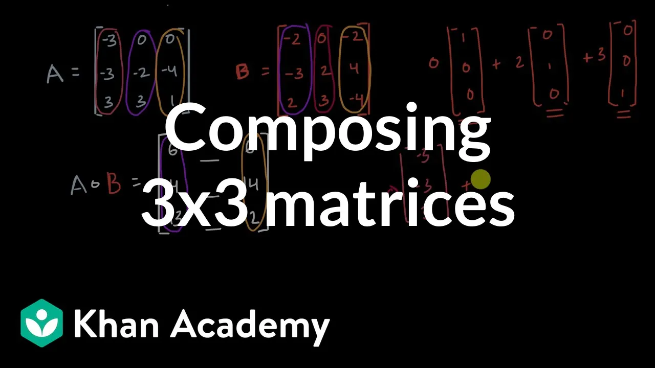
When dealing with multiple transformations, such as applying one rotation followed by another, we use matrix multiplication. Mathematically, multiplying two 3x3 matrices represents the composition of their respective spatial transformations. The rightmost matrix acts first on the initial space, followed by the leftmost matrix acting on the already transformed result. This compositional property makes 3D matrix multiplication highly valuable in practical fields like computer graphics and robotics, allowing complex movements to be broken down into simpler, sequential steps.
Knowledge cards
01
Standard Basis Vectors in 3D
In three-dimensional Cartesian space, any vector can be decomposed using three mutually orthogonal unit vectors aligned with the primary axes. They serve as the fundamental building blocks for defining linear transformations.
i^=100,j^=010,k^=001
02
Constructing Transformation Matrices
A linear transformation in 3D space is completely characterized by its effect on the standard basis vectors. The images of these basis vectors under the transformation form the columns of the associated 3x3 matrix.
T(i^)→c1,T(j^)→c2,T(k^)→c3⟹M=[c1∣c2∣c3]
03
Rotation About the Y-Axis Example
For a 90-degree rotation around the y-axis, the vertical basis vector j^ is invariant. The horizontal basis vector i^ rotates onto the negative z-axis, and the depth basis vector k^ rotates onto the positive x-axis. Their new coordinates populate the matrix columns. This uses column vectors and a positive 90° rotation by the right-hand rule in a right-handed frame. Different conventions change the signs.
Ry(90∘)=00−1010100
04
Linearity and Vector Mapping
Because linear transformations respect vector addition and scalar multiplication, mapping an arbitrary vector (x,y,z)T simply requires taking a linear combination of the matrix's columns, weighted by the input vector's components.
Mv=x(T(i^))+y(T(j^))+z(T(k^))
05
Composition of Transformations
Multiplying two matrices corresponds to executing their underlying geometric transformations sequentially. In the product AB, the transformation represented by B occurs first, altering the space, which is then subjected to the transformation represented by A.
The reviewed matrix-construction card explains that a linear map on three-dimensional space is determined by the images of its standard basis vectors, placed as matrix columns. Arbitrary inputs map by the corresponding linear combination. With column vectors, AB applies B first and then A; rotation signs depend on the stated coordinate and orientation conventions.
During a 90-degree rotation around the y-axis, i^ moves to the negative z-axis at (0,0,−1), j^ remains stationary on the y-axis at (0,1,0), and k^ swings to the positive x-axis at (1,0,0).
Conditions: Rotation angle is exactly 90 degrees; Axis of rotation is the y-axis; Right-handed coordinate system convention assumed for sign determination
Multiplying a 3x3 matrix by a vector (x,y,z) scales each column of the matrix (which represents a transformed basis vector) by the corresponding input coordinate and sums the results. This works because linear transformations preserve addition and scalar multiplication.
Conditions: Matrix is 3x3 representing a linear transformation; Input vector has coordinates (x,y,z); Transformation is linear
Matrix-vector multiplication in 3D works by scaling the columns of the matrix by the corresponding coordinates of the input vector and summing the results. The coordinates (x,y,z) act as scalar multipliers for the transformed basis vectors (the columns), leveraging the linearity property that preserves addition and scalar multiplication.
Conditions: The matrix is a 3x3 transformation matrix.; The input vector has coordinates (x,y,z).; The transformation is linear.
Multiplying two 3x3 matrices represents applying their respective spatial transformations sequentially. The rightmost matrix acts first on the initial space, and the leftmost matrix acts on the already transformed result.
Conditions: Both matrices are 3x3 transformation matrices.; The operation is standard matrix multiplication.
To construct the 3x3 matrix, observe where the three standard basis vectors (i^, j^, and k^) land after the transformation. Record the final coordinates of these transformed vectors as column vectors.
Conditions: Working in three-dimensional Cartesian space.; The transformation is linear.
When multiplying two matrices A and B to form AB, the transformation represented by the rightmost matrix B acts first on the initial space, followed by the leftmost matrix A acting on the already transformed result.
Conditions: Performing matrix multiplication AB; Matrices represent linear spatial transformations; Vectors are treated as column vectors
A 3D linear transformation is fully determined by tracking where the standard basis vectors (i^, j^, and k^) land. The coordinates of these three transformed vectors are recorded as column vectors to form a 3x3 matrix.
Conditions: Working in three-dimensional Cartesian space; Using the standard basis vectors aligned with x, y, and z axes; The transformation is linear (preserves grid lines parallel/evenly spaced and fixes origin)
The matrix is 00−1010100. This is derived by tracking the standard basis vectors: i^ moves to (0,0,−1), j^ remains stationary at (0,1,0), and k^ swings to (1,0,0).
Conditions: Rotation is 90 degrees around the y-axis.; Working in a right-handed 3D coordinate system.