Calculus / Chinese

Mean value theorems compared

Charles队长 · Bilibili · 1:04

Bilibili · Charles队长Original video

IN THIS VIDEO

01Cauchy's Mean Value Theorem
02Lagrange's Mean Value Theorem
03Rolle's Mean Value Theorem

FROM THE LEARNING NOTES

\exists \xi \in (a,b): \frac{f'(\xi)}{g'(\xi)} = \frac{f(b)-f(a)}{g(b)-g(a)}

Cauchy's Mean Value Theorem

SELECTED MOMENT

Title & Introduction

SUGGESTED PREPARATION

Geometric meaning of derivatives
Basics of parametric equations
Distinction between continuity and differentiability

READ & KEEP

The explanation, unpacked.

Saves 0

Reviewed learning material · Video analysis · English

Read the full overview

This animated video illustrates the evolutionary relationship among three fundamental Mean Value Theorems: Cauchy's, Lagrange's, and Rolle's. It begins by presenting Cauchy's theorem from a parametric curve perspective, then derives Lagrange's theorem as a specific case when $g(t)=t$ , and finally simplifies it further into Rolle's theorem under the condition $f(a)=f(b)$ . A concluding flowchart summarizes the logical progression from general principles to special cases.

Use the learning inspector for key ideas and moments, or open the reading tabs for the complete notes.

Chapters

0:00Title & Introduction 0:06Cauchy MVT via Parametric Curves 0:25Lagrange MVT as a Special Case 0:38Rolle MVT as a Further Restriction 0:50Logical Summary of Three Theorems

Learning script

Generated from the video's visuals and explanation; not verbatim speech.

This video explores the intrinsic connections between three core differential mean value theorems in mathematical analysis: Cauchy's, Lagrange's, and Rolle's. We will demonstrate that these theorems are not isolated facts but rather perfectly embody the mathematical evolution from general laws to special scenarios.

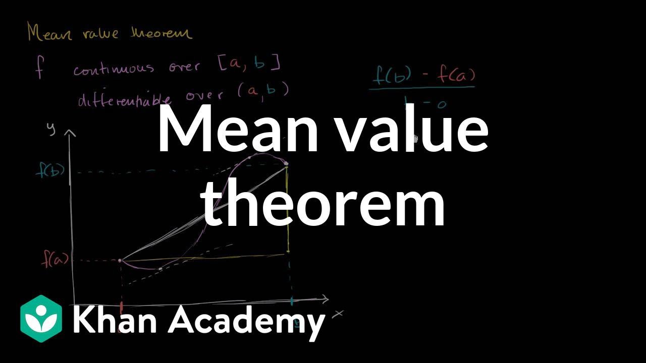
We start with the most general form: Cauchy's Mean Value Theorem. Consider a continuous differentiable curve defined by parametric equations $\gamma(t) = \begin{cases} x=g(t) \\ y=f(t) \end{cases}$ in a Cartesian coordinate system. Selecting two points $\gamma(a)$ and $\gamma(b)$ on the curve, the red chord connecting them has a slope of $\frac{f(b)-f(a)}{g(b)-g(a)}$ . According to the theorem, there must exist a point $\xi \in (a,b)$ where the tangent direction is parallel to this chord, satisfying $\frac{f'(\xi)}{g'(\xi)} = \frac{f(b)-f(a)}{g(b)-g(a)}$ . This geometric intuition reveals the profound link between the ratio of function increments and their derivatives. The ratio form additionally requires g′ nonzero throughout the open interval to avoid division by zero; a cross-multiplied form avoids that division.

Next comes the first degeneration: let the horizontal parameter be $g(t) = t$ . At this stage, the curve shape returns directly to our familiar standard function graph $y=f(x)$ without complex functional control over the coordinates. Substituting into the previous formula, since $g'(\xi)=1$ and the interval length becomes $b-a$ , the originally complicated proportion instantly simplifies to $\exists \xi \in (a,b): f'(\xi) = \frac{f(b)-f(a)}{b-a}$ . This is precisely the famous Lagrange Mean Value Theorem, indicating that for any smooth curve, there exists a point whose instantaneous rate of change equals the average rate of change across the entire interval.

Then follows the second degeneration: building upon Lagrange's theorem, we add the condition that endpoint values are equal, i.e., $f(a)=f(b)$ . This implies that the function graph starts and ends at the same horizontal height, turning the chord connecting the two points into an absolutely horizontal straight line with zero slope. Consequently, the numerator of the fraction on the right side of the equation reduces to zero, naturally contracting the conclusion to $\exists \xi \in (a,b): f'(\xi) = 0$ . This is Rolle's Mean Value Theorem, guaranteeing that if the starting and ending heights match, there must be an extremum or stationary point in between—where the tangent is completely horizontal.

Finally, we review the whole picture through a clear hierarchical structure diagram. Inside the top blue box lies the most universal Cauchy Mean Value Theorem; flowing downward after filtering through the condition ' $g(t)=t$ ', it enters the green Lagrange Mean Value Theorem box; continuing to apply the restriction ' $f(a)=f(b)$ ', it ultimately settles into the red Rolle Mean Value Theorem. This step-by-step deduction not only clarifies conceptual boundaries but also showcases the concise yet beautiful unity within the mathematical system.

Knowledge cards

Cauchy's Mean Value Theorem

The broadest mean value theorem based on the perspective of parametric curves. For two functions $f(t)$ and $g(t)$ defined on a closed interval, which are continuous there and differentiable in the open interval, provided $g'(t) \neq 0$ , there exists at least one point $\xi$ such that the ratio of their derivatives equals the ratio of their increments at the endpoints. Geometrically, this means the tangent at some point on the curve is parallel to the secant line connecting the endpoints.

\exists \xi \in (a,b): \frac{f'(\xi)}{g'(\xi)} = \frac{f(b)-f(a)}{g(b)-g(a)}

Lagrange's Mean Value Theorem

A special case of Cauchy's Mean Value Theorem. When the independent variable mapping in the parametric equations is set as the identity transformation $g(t)=t$ , the original theorem degenerates into the single-variable function format. It states that if a function is continuous on a closed interval and differentiable on the corresponding open interval, there necessarily exists a point inside the interval where the derivative exactly equals the function's average rate of change (i.e., the slope of the secant line).

\exists \xi \in (a,b): f'(\xi) = \frac{f(b)-f(a)}{b-a}

Rolle's Mean Value Theorem

If f is continuous on [a,b], differentiable on (a,b), and $f(a)=f(b)$ , some interior point has zero derivative. A stationary point is not synonymous with a local extremum; zero derivative alone does not decide extrema.

\exists \xi \in (a,b): f'(\xi) = 0 \quad (\text{given } f(a)=f(b))

Explore the knowledge in this video

Open video knowledge graph →

Mean value theorem Explanation
Why this connection?
This animated video illustrates the evolutionary relationship among three fundamental Mean Value Theorems: Cauchy's, Lagrange's, and Rolle's. It begins by presenting Cauchy's theorem from a parametric curve perspective, then derives Lagrange's theorem as a specific case when $g(t)=t$ , and finally simplifies it further into Rolle's theorem under the condition $f(a)=f(b)$ . A concluding flowchart summarizes the logical progression from general principles to special cases.
Derivatives Application
Why this connection?
This animated video illustrates the evolutionary relationship among three fundamental Mean Value Theorems: Cauchy's, Lagrange's, and Rolle's. It begins by presenting Cauchy's theorem from a parametric curve perspective, then derives Lagrange's theorem as a specific case when $g(t)=t$ , and finally simplifies it further into Rolle's theorem under the condition $f(a)=f(b)$ . A concluding flowchart summarizes the logical progression from general principles to special cases.

Mean value theorems compared

The explanation, unpacked.

Chapters

Learning script

Knowledge cards

Cauchy's Mean Value Theorem

Lagrange's Mean Value Theorem

Rolle's Mean Value Theorem

Explore the knowledge in this video

Connect the next step

In another language

A different approach