AR models use past observations
The video defines an autoregressive model as one that forecasts a series from its own past values. These past values are called lags. This distinguishes AR from MA, which uses past errors instead.
Aric LaBarr · YouTube · 5:07
This 120-second lecture segment reviews AR and MA models, shows by recursive substitution that an AR(1) model can be written as an infinite moving-average model, and then introduces the general ARMA equation combining lagged observations and lagged errors. It closes by naming two approaches for choosing ARMA orders: plotting correlation patterns and using automatic selection techniques. This video segment introduces the concept of selecting appropriate autoregressive (AR) and moving average (MA) orders for ARIMA models. It outlines three automatic selection techniques—MINIC, SCAN, and ESACF—and explains their methodologies. The segment emphasizes that these techniques serve as starting points for model building rather than definitive solutions. This introductory video explains the components of ARIMA models for time series analysis. It covers automatic selection techniques using MINIC, SCAN, and ESACF grids to identify AR and MA orders. The video then defines the 'I' in ARIMA as integrated, explaining stationarity and how differencing is used to achieve it. Finally, it breaks down the ARIMA(p, d, q) notation and provides a concrete example of constructing an ARIMA(1,1,1) model.
Use the learning inspector for key ideas and moments, or open the reading tabs for the complete notes.
Generated from the video's visuals and explanation; not verbatim speech.
The clip opens with the title question “WHAT ARE ARIMA MODELS?” and immediately frames the topic as a continuation from earlier discussions of AR and MA models.
A review slide defines the two building blocks. AR means forecasting from past observed values of the series, called lags. MA means forecasting from past errors, called error lags. The accompanying sales-versus-time chart visually anchors these ideas in a real time series.
The lecture then shifts to the relationship between the two. Starting from the AR(1) equation , the speaker explains that because itself depends on , the current value inherits dependence farther and farther back in time. This recursive backward view is why AR models are described as long-memory models.
The algebra is continued on screen: after substitution, the model is rewritten as , and then expanded further until it reaches . The important visual move is to ignore the initial-condition term and focus on the accumulated error terms.
That accumulated error piece is identified as a large moving-average component. If the recursion is not stopped at a finite starting observation, the slide summarizes the result as . In words, the video presents an AR model as an infinite MA model built from many short-memory shock effects.
The next slide interprets this conceptually: long memory in AR arises from collecting many short-memory MA effects. This motivates the practical step of combining AR and MA structures rather than relying on an extremely long pure AR or pure MA representation.
The general ARMA model is then written explicitly as . The speaker explains that ARMA models usually need fewer terms while still capturing the dynamics well.
Finally, the clip introduces the next problem: deciding how many ’s and ’s to use. Two methods are named on the slide—plotting correlation patterns and automatic selection techniques—but the explanation is cut off before either method is developed.
The video begins by addressing the challenge of determining the number of autoregressive (AR) and moving average (MA) terms, denoted as p and q respectively, in an ARIMA model.
Due to time constraints, the presenter opts for computational approaches over traditional methods like plotting autocorrelation and partial autocorrelation functions, which can become complex for intricate models.
Three primary automatic selection techniques are introduced: MINIC, SCAN, and ESACF. These methods are described as starting points for model building, encouraging further refinement through trial and error.
MINIC, or Minimum Information Criterion, involves constructing a grid of potential AR and MA orders, fitting models for each combination, and selecting the one with the lowest Bayesian Information Criterion (BIC).
SCAN, or Squared Canonical Correlations, analyzes the correlation matrix of the data and its lags, extracting eigenvalues to identify AR and MA orders that yield near-zero canonical correlations.
ESACF, the Extended Sample Autocorrelation Function, iteratively filters out AR terms until only MA components remain, ensuring that residual correlations are minimized.
The video begins by discussing automatic selection techniques for time series models, specifically mentioning MINIC, SCAN, and ESACF. Visual grids are used to illustrate how these techniques help identify the appropriate number of Autoregressive (AR) and Moving Average (MA) terms by looking for patterns like upper right triangles.
Next, the focus shifts to the 'I' in ARIMA, which stands for 'integrated'. This relates to the concept of stationarity in time series data. Stationarity is defined as the property where the data's distribution depends only on the time difference between observations, not their absolute position in time. To achieve stationarity, the video explains that differencing is typically applied to the data.
The presentation then summarizes the standard notation for ARIMA models: ARIMA(p, d, q). It clearly defines each parameter: 'p' represents the number of AR terms, 'd' is the number of first differences applied, and 'q' denotes the number of MA terms.
To solidify the concept, a specific example of an ARIMA(1,1,1) model is constructed. The process involves first taking a single difference () of the original series to create a stationary series . Then, an ARMA(1,1) model is fitted to , incorporating one autoregressive term () and one moving average error term ().
The video concludes by reiterating that these steps and definitions encompass what ARIMA models are and how they can be selected.
The video defines an autoregressive model as one that forecasts a series from its own past values. These past values are called lags. This distinguishes AR from MA, which uses past errors instead.
A moving-average model is defined as forecasting from past error terms, called error lags. The clip emphasizes that these are shocks to the series, not previous observed values.
Because an AR model can be expanded recursively backward in time, earlier observations continue to influence the present. The video uses this recursive dependence to explain the phrase long memory.
Starting from , substituting backward produces expressions involving , then earlier lags, and eventually plus a weighted sum of past errors. The slide highlights the error-sum part as the key moving-average component.
If the recursion is allowed to continue indefinitely rather than stopping at a first observation, the AR(1) model becomes an infinite moving-average model in past errors. This is the central equivalence stated in the clip.
The video interprets the AR structure as a collection of many short-memory MA effects. Each lagged error contributes a small piece, and together they generate the longer-lived dependence associated with AR models.
ARMA combines autoregressive terms in past observations with moving-average terms in past errors. The stated advantage is parsimony: one can often replace very large pure AR or pure MA models with a smaller mixed ARMA model.
After defining ARMA, the clip introduces the next task: determining how many AR and MA terms to include. Two approaches are named: plotting correlation patterns and using automatic selection techniques.
The ARIMA model integrates autoregressive (AR) and moving average (MA) components to forecast time series data. Its general form includes constants, AR terms, MA terms, and a white noise error term.
MINIC, SCAN, and ESACF are computational methods designed to assist in choosing suitable AR and MA orders for ARIMA models. They serve as initial guides rather than conclusive tools.
MINIC evaluates various AR and MA order combinations via a grid search and selects the model with the lowest Bayesian Information Criterion (BIC), providing a systematic approach to model selection.
SCAN examines the correlation matrix of the data and its lags, focusing on eigenvalues (squared canonical correlations) to pinpoint AR and MA orders that result in minimal correlations.
ESACF progressively eliminates AR terms until only MA components persist, ensuring that the remaining autocorrelations are effectively reduced, thus identifying optimal ARIMA orders.
Techniques like MINIC, SCAN, and ESACF use grids mapping AR and MA orders to suggest potential model structures. Analysts look for specific patterns, such as upper right triangles, to identify candidate ARMA(p,q) models.
A time series is stationary if its statistical properties, like mean and variance, depend only on the time lag between observations, not the specific time point. This is crucial for many forecasting models.
Differencing is a transformation applied to non-stationary time series to make them stationary. It involves calculating the difference between consecutive observations (e.g., ).
ARIMA models are parameterized by three integers: p (number of AR terms), d (degree of differencing), and q (number of MA terms).
An ARIMA(1,1,1) model first differences the original series () and then fits an ARMA(1,1) model to the differenced series, including one AR lag () and one MA lag ().
Explore conditions, steps and evidence. Supplementary explanations are labeled separately from content shown in the video.
The slide shows the dependent variable as in the AR(1) recursion and later in the general ARMA equation.
Time-series observation at time .
Observed series values used in autoregressive terms.
The slide shows , , , and later in the ARMA equation.
Error term (innovation/shock) at time .
Past errors used in moving-average terms.
The AR(1) recursion uses and , and the general ARMA formula uses .
The video does not explicitly state stationarity restrictions on .
The starred intercept is shown but not defined verbally in this clip.
, ,,
Autoregressive coefficients multiplying lagged observations.
Parameters of AR terms.
The ARMA slide displays .
The video does not explicitly state invertibility restrictions on .
No separate verbal definition of is given in this clip.
,,
Moving-average coefficients multiplying lagged errors.
Parameters of MA terms.
The speaker does not define or in words during this clip.
The exact relationship between and is not explained in the clip.
Whether equals is not stated here.
,\
Constant/intercept term in the model equations.
Additive intercept in AR and ARMA representations.
The speaker says ARMA models combine AR and MA terms and typically have fewer terms.
The clip does not formally define and as integers beyond their appearance in the formula.
p,\ q
Order parameters: for autoregressive lags and for moving-average error lags.
Model orders in ARMA notation.
Time series variable at time t
Real numbers
Constant term in the ARIMA model
Real numbers
Coefficients of the autoregressive (AR) terms
Real numbers
Coefficients of the moving average (MA) terms
Real numbers
White noise error term at time t
Real numbers
p
Order of the autoregressive (AR) part
Non-negative integers
The speaker says AR models forecast a series based solely on past values of the series, called lags.
Slide text reads: 'AR – forecast a series based solely on the past values in the series – called lags.'
An autoregressive (AR) model forecasts a time series using only its own past observed values, referred to as lags.
Forecasting a time series
Uses past values of the same series
The speaker says MA models forecast a series based on past values of the errors in the series, called error lags.
Slide text reads: 'MA – forecast a series based solely on the past errors in the series – called error lags.'
A moving-average (MA) model forecasts a time series using past error terms (shocks), called error lags.
Forecasting a time series
Uses past errors rather than past observations
The speaker says AR models are called long memory models because one can recursively look back over time and still see effects from lags.
The slide shows and then .
The clip does not state the convergence condition needed for an infinite backward expansion.
AR models are described as long-memory models because the effect of earlier observations can be traced backward recursively through lagged dependence.
Applies to autoregressive time-series models
Assumes recursive substitution backward in time
The speaker says that instead of very large AR or MA models, one can combine them into ARMA models that typically have fewer terms but model just as well.
The slide title is 'Autoregressive Moving Average Models (ARMA)' and the text says 'Have both AR and MA terms together in the model.'
The claim that ARMA models 'typically have fewer terms but model just as well' is presented qualitatively, without proof in this clip.
An ARMA model combines autoregressive terms in past observations with moving-average terms in past errors within a single equation.
Time-series modeling
Includes both lagged observations and lagged errors
The final slide lists 'Plotting patterns in correlation' and 'Automatic selection techniques' under 'Couple of different techniques to selecting models'.
The speaker begins to transition toward how to determine model order, but the sentence is cut off before explanation.
The clip ends before any method is explained in detail.
No specific correlation plots or selection criteria are shown yet.
The video introduces two ways to choose model order: plotting correlation patterns and using automatic selection techniques.
Used when deciding how many AR and MA terms to include
The ARIMA model combines autoregressive (AR) and moving average (MA) terms to model time series data. The general form is given by the equation shown.
p and q are non-negative integers
is white noise
Three common techniques are called the MINIC, SCAN, and ESACF.
MINIC, SCAN, and ESACF are computational methods used to select appropriate AR and MA orders for an ARIMA model.
Used as starting points for model building
Slide text states: 'Distribution depends only on difference in time, not location in time.'
Speaker explains that stationarity means the distribution of your data depends only on differences in time, not location in time.
In the context of time series, stationarity means that the statistical distribution of the data depends only on the difference in time between observations, rather than their absolute location in time.
Applies to time series data.
Slide text states: 'Essentially, you need to make your data stationary (typically done through differencing).'
Speaker says, 'Typically, we take differences in our data to make our data stationary.'
Differencing is a technique used to transform a non-stationary time series into a stationary one by computing the differences between consecutive observations.
Used when data exhibits non-stationarity.
The speaker says that if time is not stopped, an AR model is an infinite moving average model.
The slide title changes to 'AR(1) = MA()' and boxes the error-only part of the expanded expression.
The clip does not state the formal condition required for the infinite MA representation.
By recursively substituting lagged terms backward, an AR(1) model can be rewritten as an infinite moving-average representation in past errors.
Start from an AR(1) equation of the form .
Continue the recursion far enough back in time.
The clip leaves unstated the usual convergence/stationarity condition needed for the infinite limit.
For the AR(1) model shown, repeated backward substitution yields an expression involving infinitely many lagged error terms if time is not stopped.
The speaker says AR and MA models are essentially opposites and that collecting short-memory MA effects makes the long-memory AR effect.
The slide title reads 'Long Memory and Short Memory?' and the bottom text says 'Collection of a bunch of short memory effects!'
This is an intuitive characterization rather than a formal theorem statement in the clip.
The video presents AR and MA models as related opposites: many short-memory MA effects combine to produce the long-memory behavior associated with AR models.
Use the recursive expansion of an AR model into lagged error terms.
Interpret each lagged error contribution as a short-memory effect.
Qualitative claim about the relationship between AR and MA representations.
These techniques are just starting points though... They give you good models to start with that you can play around from there to potentially build better models.
Automatic selection techniques provide initial models that can be refined through trial and error.
Applicable to ARIMA model building
For all automatic selection techniques
The narrator explains looking back recursively until the first observation , then focusing on the right-hand side as a large moving-average term.
The algebraic derivation of from is skipped on screen.
The passage from finite to the infinite MA representation is asserted verbally rather than proved rigorously.
The clip does not mention the stationarity condition .
Begin with the AR(1) model shown on the slide.
Given model equation.
Substitute the lagged dependence backward one more step so that is expressed using and earlier errors.
Recursive substitution of the AR relation into itself.
Continue the same backward substitution repeatedly.
Iterating the recursion further back in time.
After expanding all the way back to the first observation, the expression contains a term in plus a weighted sum of past errors.
Finite backward expansion to the initial observation.
The boxed portion isolates the accumulated error terms, which the speaker identifies as a large moving-average component.
Visual emphasis on the error-only part of the expanded equation.
If the recursion is not stopped at a finite initial observation, the error expansion continues indefinitely, giving an infinite moving-average representation.
Verbal conclusion by the speaker plus slide title change.
The AR(1) model can be rewritten as an infinite moving-average model in past errors, motivating the slide statement AR(1)=MA().
The MINIC... builds many combinations of models across a grid search of AR and MA terms. It then finds the model with the lowest Bayesian information criterion.
Construct a grid of possible AR and MA orders.
Grid search approach
Fit ARIMA models for each combination in the grid.
Model fitting process
Select the model with the lowest Bayesian Information Criterion (BIC).
Optimization criterion
MINIC selects the best ARIMA model based on BIC.
The SCAN... Look at the correlation matrix of your data. Then we're going to compare that with its lags. Then we're going to look at the eigenvalues from this correlation matrix... We want to find the combination of AR and MA terms that produce canonical correlations of approximately zero.
Compute the correlation matrix of the time series data.
Correlation analysis
Compare the correlation matrix with its lagged versions.
Lag comparison
Extract eigenvalues (squared canonical correlations) from the comparison.
Eigenvalue decomposition
Identify AR and MA orders where canonical correlations approach zero.
Zero-correlation criterion
SCAN identifies suitable ARIMA models by minimizing canonical correlations.
The ESACF... We know that the AR and MA terms are related. Essentially, we're filtering out AR terms until all we have left is the MA piece. If we filter and there's still AR correlations, then we haven't filtered enough ARs out.
Filter out AR terms sequentially.
Sequential filtering
Check remaining autocorrelations after each filter step.
Residual correlation check
Continue filtering until only MA components remain.
Termination condition
ESACF determines ARIMA orders by isolating MA components through iterative AR filtering.
Slide displays ARIMA(1,1,1) with equations and .
Speaker explains that for an ARIMA(1,1,1), we first take a difference () to go from Y to W, then have a lag of , and a lag of error ().
Apply first-order differencing () to the original time series to obtain the stationary series .
Definition of differencing for stationarity.
Model the differenced series using an ARMA(1,1) process, incorporating one AR term () and one MA term ().
Definition of ARMA(p,q) model applied to the differenced series.
An ARIMA(1,1,1) model consists of taking a first difference of the original series and then fitting an ARMA(1,1) model to the resulting differenced series.
Here's one at an AR3 MA0 model. Here is another at an AR2 MA2 model. And here is yet another at an AR0 MA3 model.
Identify valid ARIMA models using SCAN method.
Correlation matrix and its lags
Find AR and MA orders with near-zero canonical correlations.
Examine correlation matrices for patterns.
Visual inspection
Identify rectangles indicating low canonical correlations.
Pattern recognition
Valid models include AR(3,0), AR(2,2), and AR(0,3).
Models show minimal canonical correlations.
Slide explicitly shows the title 'ARIMA(1,1,1)' and the corresponding equations.
Speaker says, 'So if we had an ARIMA 1 1 1, we have the following...'
Construct the mathematical representation of an ARIMA(1,1,1) model.
(one AR term)
(one first difference)
(one MA term)
Write the equations defining the ARIMA(1,1,1) process.
Take the first difference of the original series .
indicates one order of differencing.
Write the ARMA(1,1) equation for the differenced series .
and indicate one autoregressive term and one moving average term.
The ARIMA(1,1,1) model is defined by the system: and .
Matches the visual equations and audio explanation provided in the video.
A slide titled 'Remember AR and MA Models?' shows a time-series chart with y-axis 'Sales ($ Millions)' and x-axis dates from to .
Around 21s and again around 28s, orange circles highlight points on the chart while the speaker reviews AR and MA definitions.
The chart illustrates lag/error concepts visually, but the exact numerical values of the highlighted points are not discussed verbally.
Line chart of sales over time
Orange highlight circles
Bullet text defining AR and MA
Static chart remains on screen while orange circles appear around selected points.
Slide focus shifts from AR bullet to MA bullet.
The axes remain 'Sales ($ Millions)' versus dates.
The textual definitions of AR and MA stay visible.
The visual supports the verbal distinction between using past observations (lags) and past errors (error lags) in forecasting.
Slides progress from 'Relationship Between AR and MA' to 'Keep Doing Math...' to 'AR(1) = MA()' to 'Long Memory and Short Memory?' while retaining the same recursive equations.
An orange curved arrow links the first AR equation to the substituted second equation; later an orange box highlights the error-sum portion.
The intermediate algebra producing is not shown step by step.
AR(1) equation
Substituted equation with
Ellipsis line
Expanded equation ending in and error terms
Orange arrow and orange box
Equations accumulate downward as the recursion is extended.
Title changes from relationship framing to 'Keep Doing Math...', then to 'AR(1) = MA()', then to 'Long Memory and Short Memory?'.
The error-only tail is boxed for emphasis.
The core model remains an AR(1) equation being rewritten.
The left-hand side stays throughout.
The animation visually demonstrates that repeated substitution turns lagged observations into a growing weighted sum of past errors.
Three grids labeled MINIC, SCAN, ESACF showing AR vs MA orders.
MINIC grid
SCAN grid
ESACF grid
Highlighting of specific cells in grids
Grid structure remains constant
Each grid represents a different method for evaluating ARIMA model orders.
Three 5x5 grids labeled MINIC, SCAN, and ESACF are shown, with axes labeled AR (0-4) and MA (0-4). Different cells are shaded to indicate possible model orders.
MINIC grid
SCAN grid
ESACF grid
AR axis
MA axis
Shaded cells
Slide transitions from selection grids to the stationarity slide.
Axes remain AR (0-4) and MA (0-4) across all three grids.
The shaded regions in each grid represent the combinations of AR and MA orders suggested by the respective automatic selection technique. The speaker notes looking for upper right triangles and their points to identify models like ARMA(1,1), ARMA(2,2), etc.
Slide displays 'ARIMA(p, d, q)' with arrows pointing to definitions for p, d, and q.
ARIMA(p, d, q) text
Arrows
Labels for p, d, q
Slide transitions from stationarity to ARIMA notation.
Visually decomposes the ARIMA acronym, linking each parameter (p, d, q) to its specific meaning in the model structure.
Slide displays 'ARIMA(1,1,1)' with two equations below it, connected by arrows indicating the flow from to and then the ARMA equation.
ARIMA(1,1,1) text
Differencing equation
ARMA equation
Connecting arrows
Slide transitions from general notation to specific example.
Illustrates the step-by-step construction of an ARIMA(1,1,1) model, showing how differencing creates a new series which is then modeled using ARMA terms.
The speaker explicitly contrasts AR models, which use past values called lags, with MA models, which use past errors called error lags.
The slide separates the two definitions in parallel bullets.
One might think AR and MA models differ only in name, or that both use the same kind of past information.
AR models use past observed values of the series; MA models use past error terms (shocks) of the series.
The speaker says AR models are long-memory models and then explains that they can be viewed as collections of short-memory MA effects.
The slide title 'Long Memory and Short Memory?' and the boxed error sum support this interpretation.
The clip gives intuition rather than a formal memory-decay analysis.
One might think 'long memory' means the model only depends on one distant lag.
Here long memory means the recursive AR structure lets many past shocks accumulate, producing an effectively infinite MA representation.
These techniques are just starting points though... They give you good models to start with that you can play around from there to potentially build better models.
Automatic selection techniques provide final optimal models.
They offer initial models that require further refinement.
The speaker says ARMA models combine AR and MA terms together.
The ARMA equation contains both and terms.
The ARMA model includes autoregressive terms as one component of its general form.
The speaker says ARMA combines AR and MA models into one framework.
The ARMA equation includes lagged error terms with coefficients .
The ARMA model includes moving-average terms as the other component of its general form.
The slide title becomes 'AR(1) = MA()' after the recursive expansion.
The speaker states that an AR model is an infinite moving average model if time is not stopped.
The formal condition for equivalence is omitted in the clip.
The long-memory AR representation is shown to be equivalent, under the video's recursive argument, to an infinite MA representation.
The slide 'Deciding How Many p's and q's...' appears directly after the ARMA definition slide.
The speaker transitions from defining ARMA to asking how to determine the model order.
The actual selection procedures are not yet explained in this clip.
Once ARMA models are defined, the next issue is choosing the orders and .
Deciding how many p's and q's... Couple of different techniques to selecting models...
Automatic selection techniques apply to determining parameters in ARIMA models.
Speaker connects making data stationary with taking differences.
Slide text links 'make your data stationary' with '(typically done through differencing)'.
Differencing is a method applied to achieve stationarity in time series data.
ARIMA(p,d,q) notation includes 'd' for first differences, and the ARIMA(1,1,1) example shows the differencing equation.
The derivation and understanding of the ARIMA model rely on the concept of differencing to handle non-stationary data.
The ARMA equation is displayed on screen.
The speaker defines ARMA as combining AR and MA terms.
The speaker calls AR models long memory models and explains recursive backward dependence.
The recursive expansion slides show rewritten in terms of earlier and values.
The slide separately defines AR and MA using lags versus error lags.
The speaker contrasts past values with past errors.
The final slide lists two techniques for selecting models.
The speaker begins transitioning to how to determine model order before the clip ends.
Only the names of the techniques are present; no detailed method is shown.
How do I decide the number of AR and MA terms in an ARIMA model?
Speaker defines stationarity.
Slide text defines stationarity.
Speaker explains differencing to make data stationary.
Slide text mentions differencing for stationarity.
Speaker defines p, d, and q.
Slide visually breaks down ARIMA(p,d,q).
Speaker walks through the ARIMA(1,1,1) example.
Slide shows the equations for ARIMA(1,1,1).
Covered · Title card 'WHAT ARE ARIMA MODELS?' with no mathematical content beyond topic introduction.
Covered · Review slide defines AR as using past values (lags) and MA as using past errors (error lags), with a sales time-series chart.
Covered · Slide 'Relationship Between AR and MA' and 'Keep Doing Math...' introduce recursive substitution of the AR(1) model.
Covered · Slide 'AR(1) = MA()' and 'Long Memory and Short Memory?' emphasize the infinite moving-average interpretation of AR.
Covered · General ARMA equation is shown and verbally motivated as a combination of AR and MA terms.
Covered · Final slide introduces two model-selection approaches: correlation plotting and automatic selection techniques.
Covered · Introduction to ARIMA model structure
Covered · Explanation of automatic selection techniques
Covered · Discussion of automatic selection techniques (MINIC, SCAN, ESACF) using grids to identify ARMA model orders.
Covered · Explanation of the 'I' in ARIMA, defining stationarity and the use of differencing to achieve it.
Covered · Breakdown of the standard ARIMA(p, d, q) notation and the meaning of each parameter.
Covered · Detailed example of constructing an ARIMA(1,1,1) model, showing the differencing step and the subsequent ARMA equation.
Covered · Closing remarks summarizing the video's content on ARIMA models and selection.
Reviewed English material v1: card/concept_card "ARIMA Model Definition" starting at 2:00 — The ARIMA model integrates autoregressive (AR) and moving average (MA) components to forecast time series data. Its general form includes constants, AR terms, MA terms, and a white noise error term.
Reviewed English material v1: card/concept_card "Stationarity in Time Series" starting at 4:11 — A time series is stationary if its statistical properties, like mean and variance, depend only on the time lag between observations, not the specific time point. This is crucial for many forecasting models.
An ARMA model combines autoregressive terms in past observations with moving-average terms in past errors within a single equation. The general equation is .
Conditions: Time-series modeling; Includes both lagged observations and lagged errors
Two methods are introduced for selecting model order: plotting patterns in correlation and using automatic selection techniques.
Conditions: Used when deciding how many AR and MA terms to include
Differencing is a technique used to transform a non-stationary time series into a stationary one by computing the differences between consecutive observations.
Conditions: Used when data exhibits non-stationarity.
In ARIMA(p, d, q), p represents the number of autoregressive (AR) terms, d is the number of first differences applied to make the data stationary, and q denotes the number of moving average (MA) terms.
Conditions: Applies to ARIMA model notation.
Stationarity means that the statistical distribution of the data depends only on the difference in time between observations, rather than their absolute location in time.
Conditions: Applies to time series data.
AR models forecast a series based solely on past values of the series, called lags. MA models forecast a series based solely on past errors in the series, called error lags.
Conditions: Forecasting a time series; Uses past values of the same series for AR; Uses past errors for MA
AR models are called long memory models because one can recursively look back over time and still see effects from lags. The effect of earlier observations can be traced backward recursively through lagged dependence.
Conditions: Applies to autoregressive time-series models; Assumes recursive substitution backward in time
An ARIMA(1,1,1) model consists of taking a first difference of the original series and then fitting an ARMA(1,1) model to the resulting differenced series. The equations are and .
Conditions: (one AR term); (one first difference); (one MA term)
 YouTube9:25
Another explanation of Time series and exponential smoothing.
Time series and exponential smoothingAnother explanation of ARIMA and differencing.
ARIMA and differencing YouTube3:07
Another explanation of Time series and exponential smoothing.
Time series and exponential smoothingAnother explanation of ARIMA and differencing.
ARIMA and differencing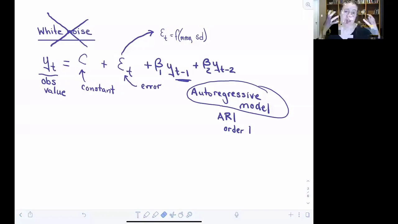 YouTube6:47
Another explanation of ARIMA and differencing.
ARIMA and differencingAnother explanation of Time series and exponential smoothing.
Time series and exponential smoothingYouTube9:25Prerequisite in Mathematical modeling: Time series and exponential smoothing → ARIMA and differencing.
Time series and exponential smoothing · View learning sequenceNext in Mathematical modeling: Time series and exponential smoothing → ARIMA and differencing.
ARIMA and differencing · View learning sequenceYouTube3:07Prerequisite in Mathematical modeling: Time series and exponential smoothing → ARIMA and differencing.
Time series and exponential smoothing · View learning sequenceNext in Mathematical modeling: Time series and exponential smoothing → ARIMA and differencing.
ARIMA and differencing · View learning sequenceYouTube6:47Next in Mathematical modeling: Time series and exponential smoothing → ARIMA and differencing.
ARIMA and differencing · View learning sequencePrerequisite in Mathematical modeling: Time series and exponential smoothing → ARIMA and differencing.
Time series and exponential smoothing · View learning sequenceYouTube9:25Whiteboard for Time series and exponential smoothing, compared with the current lecture.
Time series and exponential smoothingWhiteboard for ARIMA and differencing, compared with the current lecture.
ARIMA and differencingYouTube3:07Visual explanation for Time series and exponential smoothing, compared with the current lecture.
Time series and exponential smoothingVisual explanation for ARIMA and differencing, compared with the current lecture.
ARIMA and differencingYouTube6:47Whiteboard for ARIMA and differencing, compared with the current lecture.
ARIMA and differencingWhiteboard for Time series and exponential smoothing, compared with the current lecture.
Time series and exponential smoothing